- Research
- Open access
- Published:
Model-based learning of information diffusion in social media networks
Applied Network Science volume 4, Article number: 111 (2019)
Abstract
Social networks have become widely used platforms for their users to share information. Learning the information diffusion process is essential for successful applications of viral marketing and cyber security in social media networks. This paper proposes two learning models that are aimed at learning person-to-person influence in information diffusion from historical cascades based on the threshold propagation model. The first model is based on the linear threshold propagation model. In addition, by considering multi-step information propagation in one time period, this paper proposes a learning model for multi-step diffusion influence between pairs of users based on the idea of random walk. Mixed integer programs (MIP) have been used to learn these models by minimizing the prediction errors, where decision variables are estimations of the diffusion influence between pairs of users. For large-scale networks, this paper develops approximate methods for those learning models by using artificial neural networks to learn the pairwise influence. Extensive computational experiments using both synthetic data and real data have been conducted to demonstrate the effectiveness of the proposed models and methods.
Introduction
The rapid development of the Internet and its mobile computing technologies in the past several decades contributes to form online virtual communities in social media networks. People share news, their ideas, interests and information in social media networks. Understanding how the information propagates is essential for successful applications of viral marketing (Domingos 2005) and cyber security (Budak et al. 2011) in social media networks. To this end, researchers have defined different problems such as the influence maximization problem (Kempe et al. 2003; Kimura et al. 2007) and contamination minimization problem (Kimura et al. 2009). Influence maximization problem involves finding a limited number of nodes which have the largest influence. Similarly, contamination minimization problem involves blocking a limited number of nodes which suppress the propagation of the rumors. However, all of the parameters in the diffusion models are assumed to be known. In reality, these parameters are not readily available from the massive historical datasets of social media networks. To fill this gap, this paper proposes several models to learn these influence parameters from historical cascades.
In the literature, researchers have tried to learn the information diffusion processes through different diffusion models. There are two most prevalent diffusion models - Independent Cascade Model (IC) (Kempe et al. 2003) and General Threshold Model (GT) (Granovetter 1978). In the Independent Cascade Model, each active parent node i has a single chance to activate the child node j with a diffusion probability pi,j. Satio et al. (2008) studied the problem of learning influence probabilities based on the IC propagation model. They estimated the diffusion probabilities by expectation-maximization algorithm where the likelihood was maximized by iteratively updating the parameters. Besides, there are some variants of Independent Cascade model based research, considering continuous time delays of infection as well (Saito et al. 2009; Rodriguez et al. 2011). In contrast to IC models, General Threshold Model assumes that an inactive user j in social media networks is activated by all of its active neighbors when the total influence is larger than the target user’s threshold. Linear Threshold Model is a special case of General Threshold Model and the total influence is the sum of the influence weights of activated neighbors. Goyal et al. (2010) adopted the General Threshold diffusion Model and proposed three probabilistic models, which were Bernoulli distribution, Jaccard Index and Partical Credits to predict the diffusion influence weights. (Vaswani S, Duttachoudhury N: Learning influence diffusion probabilities under the linear threshold model, unpublished) learned the influence diffusion weights under the Linear Threshold Model. They used three different methods, i.e, gradient descent, interior point method and EM algorithm to maximize the likelihood estimate.
In this paper, we propose two different mixed-integer programming models to estimate the diffusion influence weights between pairs of users underlying the threshold model. We learn the diffusion influence weights through mining past diffusion cascades of posts. Given the historical information cascading data containing the initial states \(x_{i}^{0}\) and final states \(x_{i}^{T}\) of all the nodes which are users in social media networks, we are trying to learn the diffusion influence weights wi,j between pairs of users in the Threshold Models. Two different learning models are built under the assumption. The first model is based on the Linear Threshold Model, where a user will be activated when the sum of its neighbors’ influence weight is larger than the threshold of the user. The second model considers multi-step influence from the multi-hop neighborhood of the user. In the real dataset, the status of nodes at each time step could be collected. However, the time required for each propagation varies. When we know the status of users at two different time steps, the propagation steps could be more than one. Therefore, it’s necessary to consider multi-step influence to better fit the real data.
We summarize the contributions of this paper as follows,
We propose two mixed-integer programming models to learn diffusion influence between pairs of users. One is based on the popular propagation model, i.e., Linear Threshold Model, and another one is based on the idea of random walk considering multi-step influence.
For large-scale network, we come up with approximate methods for the two learning models using artificial neural networks with no hidden layer.
Experiments for assessing the validity of these learning models and approximate neural network methods are performed on both synthetic data and real data.
The remainder of the article is organized as follows. “Learning Models of Information Diffusion Influence” section introduces two different learning models for information diffusion prediction. “Approximate Approaches using Artificial Neural Networks” section provides approximate methods for learning models using artificial neural networks. “Experimental Evaluation” section proceeds with experimental evaluation on both synthetic data and real data. “Conclusions” section concludes the study.
Learning Models of Information Diffusion Influence
We model a social media network as a directed network G=(V,E), where V={v1,…,vn} is the set of users of the network and E⊆V×V is the set of edges representing the friend relationships between users. We observe multiple cascades spreading over it. For any information cascade propagating over the social media network, we observe the status \(x_{i}^{T}\) of each user i (i∈V) at time t=0 and t=T. The status of users is either active in reposting messages or inactive in reposting. Through mining the historical cascades, we could learn the diffusion influence weights wi,j representing the influence exerted by user i to user j in the social media network. Our model aims at learning the diffusion influence weights wi,j from user i to user j (i,j∈V) based on transitions of activation status of all users, i.e., \(x_{i}^{0}\) and \(x_{i}^{T}\) for all i∈V. To learn the diffusion influence weights, we can use a minimization model with the weights as decision variables and the objective function as the mean squared error between the predicted final status and the actual final status of users. Here we formulate two different mixed-integer programming learning models to make the prediction where the activation status is modeled by a binary variable.
Linear Threshold Learning Model
The first formulation of Linear Threshold Learning Model (LT) we come up with is underlying the Linear Threshold Propagation Model. In the propagation model of Linear Threshold Model (Chen et al. 2013; Kempe et al. 2003), initially, each node j∈V independently selects a threshold θj uniformly at random in the range of [0,1]. If the total influence weights of the arcs from its active in-neighbors \(N^{in}_{A}(j)\) is at least θj, i.e., \({\sum \nolimits }_{i\in N^{in}_{A}(j)}\omega _{i,j} \ge \theta _{j}\), then user j is activated. The diffusion influence weights are normalized in the Linear Threshold Model.
We formulate a mixed integer programming model shown below to learn the information diffusion influence between each pair of user i and user j based on the Linear Threshold Model. The objective is to minimize the mean squared error between actual final status of users and predicted final status of users. Here, the mean squared error is a quadratic function. It’s hard for solver to handle quadratic function. We linearize the objective function by replacing mean squared error with mean absolute value of the error. The mean absolute value of the error equals to the mean squared error because the status of users is a binary variable. The Constraints (1a) and (1b) represent the mean absolute error. The Constraints (1c) and (1d) represent when the total influence from its active neighbors is larger than the threshold of target user, the target user will be activated. Otherwiese, the target user will remain inactive. The Constraints (1e) represent the sum of the diffusion influence from neighbors to user j is at most 1. Constraints (1f) show when two users are connected, the value of diffusion influence is between 0 and 1. However, when they are not connected, the diffusion influence weights wi,j will be 0, which is shown in the Constraints (1g).
Where index k represents different observation, index i,j represent different users, ωi,j represents the diffusion weight from user i to user j, θj represents the threshold of user j, \(\hat {x}_{i}^{k,0}\) and \(\hat {x}_{j}^{k,T}\) are the initial status of user i and final status of user j of observation k which are known already and \(x_{j}^{k,T}\) represents the predicted final status of user j of observation k. T is the set of (j,k), where the initial status of user j of observation k denoted as \(\hat {x}_{j}^{k,0}\) should be 0. E represents the arcs of the social network.
Random Walk Learning Model
The second formulation is based on the idea of random walk. In comparison with the first formulation (LT) which considers the diffusion influence from one-step neighborhood only, Random Walk Learning Model (RW) introduces the diffusion influence from multi-step neighborhood. In reality, when we know the initial and final status of each user, we can’t tell how many steps of information propagation occur. The target node j could be activated by either one step neighborhood or even multiple step neighborhood. Therefore, we come up with a learning model considering multi-step diffusion influence between pairs of users based on the idea of random walk. Here we consider the diffusion influence from two-hop neighborhood. The total diffusion influence matrix Yk for observation k could be represented as:
Where ∘ represents the Hadamard product, A is the adjacency matrix of the social network, the (i,j) entry of A, denotes ai,j,1, is the number of paths of length 1 starting at i and ending at j. The (i,j) entry of A2, denotes ai,j,2, is the number of paths of length 2 starting at i and ending at j. W1 is the average diffusion influence weight matrix for one step diffusion, the entry ωi,j,1 denotes the diffusion influence weight from user i to user j for each one step path. W2 is the average diffusion weight matrix for two step diffusion, the entry ωi,j,2 denotes the average diffusion influence weight from user i to user j for each two step path. \(\hat {X}^{k,0}\) is a vector containing all the users’ initial status from observation k, the i entry of \(\hat {X}^{k,0}\), denotes \(\hat {x}^{k,0}_{i}\), is the initial status of user i from observation k. The learning formulation based on Random Walk is shown below:
The Constraints (3c) represent when the total influence from two step neighborhood is larger than the threshold of target user, the target user will be activated. Constraints (3d) represent when the total influence from two step neighborhood is smaller than the threshold of user, the user will not be activated. Constraints (3e) show that the average influence weights for different step of path are in the range of 0 and 1.
Approximate Approaches using Artificial Neural Networks
In the previous section, we formulate two different mixed integer programming learning models to learn the information diffusion influence weights. We could use solver Gurobi to solve the models and get a global optimal estimation of diffusion weights between pairs of users with the assumption. However, sometimes it doesn’t seem to allow for an efficient solution for large network. Here we come up with approximate approaches of Linear Threshold Learning Model and Random Walk Learning Model using artificial neural networks.
We are using the simplest kind of neural network called a single-layer perceptron network consisting of a single layer of output nodes (Bishop 2006). Then the inputs are fed directly to the outputs via a series of weights. To train the neural network and get the estimation of weights, the loss function we use is the mean squared error for both of the models. The optimization algorithm we use for training the neural network is gradient descent. Gradient descent starts with the initial values of parameters and iteratively moves toward the set of values minimizing the loss function through taking steps proportional to the negative of the gradient (Avriel 2003). To compute the gradients, backpropagation algorithm is introduced (Goodfellow et al. 2016). However, the gradient descent with backpropagation is not guaranteed to find the global optimal of the loss function.
Artificial Neural Network for Linear Threshold Learning Model
We build the Linear Threshold Neural Network (LTNN) shown in Fig. 1 to approximate the Linear Threshold Learning Model. The input \(x_{1}^{0},x_{2}^{0},\ldots,x_{n}^{0}\) are the status of n users in social media networks at time t=0. The output layer outputs \(x_{1}^{T},x_{2}^{T},\ldots,x_{n}^{T}\), which are the status of n users in social media networks at time t=T.

Neural Network for Linear Threshold Model
There are several constraints to consider for the Linear Threshold Learning Model. Firstly, if the user is active in the beginning (\(\hat {x}_{j}^{0}=1\)), then they will stay active (\(\hat {x}_{j}^{T}=1\)). To satisfy this constraint, we set the (i,j) entry of the neural network weights matrix W′, denoted as \(w^{\prime }_{i,j}\), as 1 when i equals j. In this case, when user is active at the beginning, the total influence it gets at time t=T will definitely be larger than its threshold and the user will stay active. Besides, the influence weights should be suppressed to 0 when the pair of users has no connection. Here, we use the Hadamard product of adjacency matrix A of the network and neural network weights matrix W′ to suppress the influence weights matrix W. Thirdly, in the Linear Threshold Model, the diffusion influence weights should be normalized as well. All of the constraints above could be satisfied by designing the structure of neural network. However, the Linear Threshold Model has the activation function of step function. The gradients of step function are vanishing and the weights will not update at all (Friesen and Domingos 2017). The neural network is using gradient to update the estimation. Therefore, step function is not applicable to neural network. Instead, we approximate the step function using sigmoid function. Then the output \(X^{T}=\left \{x_{1}^{T},x_{2}^{T},\ldots,x_{n}^{T}\right \}\) of neural network could be represented as:
Where θ is the threshold vector of users and I is the identity matrix. As mentioned before, the influence weights are normalized as well, thus the diffusion influence weight ωi,j(ωi,j∈W) between user i and user j could be represented as:
Where aij is the (i,j) entry of adjacency matrix A and \(\phantom {\dot {i}\!}\omega _{ij}^{\prime }\) is the (i,j) entry of artificial neural network weights matrix W′.
Artificial Neural Network for Random Walk Learning Model
The structure of neural network called Random Walk Neural Network (RWNN) built for Random Walk Learning Model is shown in Fig. 2. Here we consider the diffusion influence could be from 2-step neighborhood. Therefore, the input is the two times combination of the initial status of n nodes, denoted as \(x_{1}^{0},\ldots,x_{n}^{0},x_{1}^{0},\ldots,x_{n}^{0}\). The output layer outputs \(x_{1}^{T},x_{2}^{T},\ldots,x_{n}^{T}\), which are the status of users in the social media at time t=T.

Neural Network for Random Walk Learning Model
To satisfy the constraints in Random Walk Learning Model, we make the following modifications to the artificial neural network. Considering the diffusion influence from two step neighborhood, the total influence shown in Eq. 1 in the Random Walk Model could be transferred as:
Besides, the user will remain active when they are active in the beginning. Thus we add the identity matrix I to adjacency matrix A to satisfy the constraint. Then the output vector \(X^{T}={x_{1}^{T},x_{2}^{T},\ldots,x_{n}^{T}}\) of neural network could be represented as:
Where θ is the threshold of users, A is the adjacency matrix, A2 is the square of adjacency matrix. \(W_{1}^{\prime }\) and \(W_{2}^{\prime }\) are weights matrix of neural network. Thus the diffusion influence weights matrix W could be represented as:
Experimental Evaluation
In this section we conduct the experimental evaluation of our proposed models which are Linear Threshold Model, Random Walk Model, Linear Threshold Neural Network Model and Random Walk Neural Network Model to learn the information diffusion weights. We analyze the performance of proposed models on both synthetic data and real data.
Experiments on Synthetic Data
Firstly, we generate synthetic data to evaluate our models. The generation of synthetic data includes both network generation and cascade generation.
Network generation: In order to understand how the underlying network topology affects the performance of our learning models, we generate different well-known generative networks.
Erdos-Renyi Graph: In the graph theory, Erdos-Renyi model generates random graph. Here we use the G(n,p) model in which a graph is constructed by connecting nodes randomly by edges with probability p. For experimental purpose, we generate the network shown in Fig. 3 containing 50 nodes and generate edges between each pair of nodes in the network with probability of 0.3.
Fig. 3 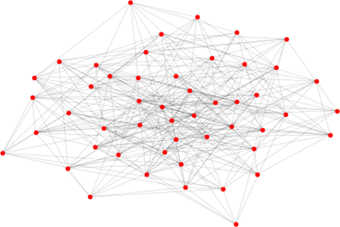
Erdos-Renyi
Barabasi-Albert Graph: Social media networks are thought to be scale-free. Barabasi-Albert graph generates random scale-free networks using a preferential attachment mechanism. Here we generate a graph of 50 nodes shown in Fig. 4 which is grown by attaching new nodes each with 15 edges that are preferentially attached to existing nodes with high degree.
Fig. 4 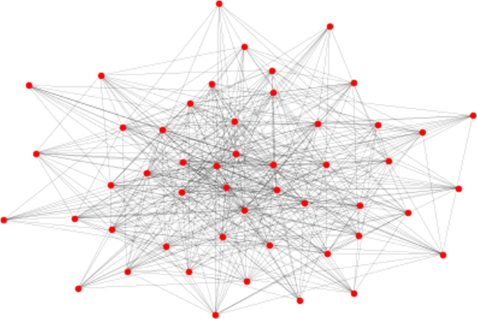
Barabasi-Albert
Watts-Strogatz Graph: Watts-Strogatz model generates random graph with small-world properties, which are short average path lengths and high clustering. Here we generate a graph of 50 nodes shown in Fig. 5, and each of them connects to 15 nearest neighbors. In addition, the probability of rewiring each edge is 0.5.
Fig. 5 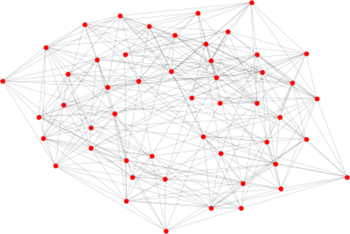
Watts-Strogat


Cascade generation: We learn the diffusion influence weights from mining historical diffusion cascades. Here, we generate the cascades for the synthetic data. We randomly select a set of seed nodes accounting for 35% of total nodes. Then the seed nodes could propagate the information to other nodes. Here we assume the active nodes will remain active and the inactive nodes will have the chances to be activated only when they have connections to active nodes within 2 step neighborhood. The activation probability p for target node is defined as:
Where N represents the total number of nodes and AN represents the active direct neighbors. We set a as 0.5 and b as 0.5 for the following experiments. We experiment with 200 cascades to compare the performance of different learning models.
Implementation Details and Evaluation: In order to learn the diffusion influence weights under different proposed learning models, we set the threshold of 0.5 for each user in the social media network. In order to provide an unbiased evaluation of a final model on the training dataset, we split the dataset into training set and testing set with 80% of training set and 20% of testing set. To validate the performance of the mixed integer programming learning models and the approximate neural network learning models, we evaluate the performance of accuracy. Accuracy is the ratio of correct predictions. Regarding to solve the problem using mixed-integer programming, we propose the decomposition method which is tractable to compute and to optimize for the original learning models. For each node, we apply the optimization model to get the diffusion weights separately because the diffusion influence from neighbors to each node is independent from each other. For the neural network learning models, we train in 10000 steps, with batch size of 10 and learning rate of 0.001.
Experimental Results: For different network types, we generate the same number of cascades using the same cascade generation strategy to compare the performance of different models. Table 1 shows the performance of synthetic data of 50 nodes.
The performance of different learning models are consistent in different network topologies. For the same number of observations(cascades), approximate neural network learning methods even outperform the mixed integer programming learning methods. The mixed integer programming methods of Linear Threshold Model and Random Walk Model have severe overfitting problems. In addition, the computational time for mixed integer programming models is much longer than neural network based models.
Therefore, for larger scale networks we conduct the experimental evaluation just using approximate neural network learning models. The performance of different sizes of networks which are 100 nodes and 1000 nodes are shown in Table 2. The testing accuracy is consistent for different network types.
The performance of different models could be affected by the way of generating cascades. We test the performance of different generation methods by changing a and b parameters in Eq. 4 using the same network topology. The performance of different network topologies are shown in Figs. 6, 7 and 8. When a is larger which means getting more influence from two step neighborhood, Random Walk Neural Network Model outperforms Linear Threshold Neural Network Model.

Erdos-Renyi

Barabasi-Albert

Watts-Strogat
Experiments on Real Data
We collect the real data from Lerman Digg 2009 dataset (Lerman and Ghosh 2010). The Digg 2009 dataset contains data about stories promoted to Digg’s front page over a period of a month in 2009. The dataset contains the time stamp of all of the users’ vote for the stories. Both of the network topology and cascade information can be obtained from the dataset.
Dataset Preprocessing: Considering the computation limitation of mixed integer programming models, we extract a small size subgraph containing 1203 nodes shown in Fig. 9 to compare the performance between mixed integer programming learning models and approximate neural network learning models. Our extracted subgraph contains 1203 users shown in Fig. 9. In Fig. 10, we could see the degree distribution of all the users follows power law distribution. The extracted network keeps the social network property of scale-free. In addition, to prove the effectiveness of the proposed models in large scale social network, we extract a network with 42259 nodes and conduct the experiments using neural network based models. In order to get the cascade information, we choose the most voted 600 stories. Then we collect all the users voting status at time T0 and Tt for each story.

Network Topology

Degree Distribution
Implementation Details and Evaluation: To investigate the performance on real data, we set the threshold of 0.5 for each user in each of the proposed learning models.
Experimental Results of Real Data: We proceed with experiments on preprocessed real data of 1203 nodes to see the performance of different learning models. We collect the historical cascades of 650 stories and get 406 efficient cascades. We treat 300 observations as training samples and the rest of observations as testing samples. For the neural network models, we train in 10000 steps with batch size of 10 and learning rate of 0.001. The performance of the dataset is shown in Table 3. First, we evaluate the performance of different learning models based on test accuracy. Random walk learning model has the best performance in this preprocessed real dataset. It doesn’t have any overfitting issue here which is likely due to the fact of sparseness of the network. In general, the random walk based learning models outperform the linear threshold based learning models in this preprocessed dataset. However, when it comes to the speed of computation, the approximate methods using neural network, i.e., LTNN and RWNN are much faster.
Then, we examine the performance of LTNN model and RWNN model using cascade information from different time intervals. We collect the data from different lengths of time intervals. One has the time interval of 4T0 and another has the time interval of 9T0. Figure 11 shows the performance comparison of two approximate models during different time intervals. For shorter time period, the LTNN model has significant improvement over RWNN model. In converse, RWNN model outperforms LTNN model in longer time period. This happens because in short time period, only one step propagation could happen. In longer time period, two-steps or multiple steps propagation could occur where random walk based model would better describe the information diffusion process.

Performance of Different Time Intervals
For the large scale network containing 42259 users, we collect the historical cascades of 600 stories and get 566 efficient casacades for experimental purpose. We treat 440 cascades as training samples and the rest as testing samples. We train in 500 steps with batch size of 10 and learning rate of 0.001. The cascade has the time interval of 9T0. The experimental result of the large dataset is shown in Table 4. Random Walk Neural Network Model requires 380GB memory and it takes about 10 min for each step. It’s time consuming and it gets stuck during the optimization process because of too many nodes. In comparison, Linear Threshold Neural Network Model converges in 500 steps and has very good performance.
Conclusions
We have investigated the problem of learning diffusion influence weights between pairs of users in social media networks from mining historical cascades. We formulate two different mixed-integer programming models to learn the diffusion influence weights which could be used to predict the status of users in the future. The first mixed integer programming model is based on the popular propagation model, i.e., Linear Threshold Model. The second mixed integer programming model is based on the idea of random walk considering the influence from multi-step neighborhood. For larger network, we introduce approximate approaches for both models using neural network. We bring marriage between optimization-based diffusion models and deep neural network through approximating optimization models using deep neural networks. Therefore, the parameters in the neural network are explainable, which are diffusion weights related parameters in our models. The approximate approaches using artificial neural networks have relatively good performance and fast computational speed.
There are several interesting directions for future works. Here we just learn the information diffusion influence through the historical cascades. It would be more interesting to consider other features such as the similarity between posters and reposters, the user profiles or even the topology information of the social media networks to make predictions with higher accuracy.
Availability of data and materials
Data is available on request from corresponding author.
References
Avriel, M (2003) Nonlinear programming: analysis and methods. Courier Corporation, Mineola.
Bishop, CM (2006) Pattern recognition and machine learning. Springer, New York.
Budak, C, Agrawal D, El Abbadi A (2011) Limiting the spread of misinformation in social networks In: Proceedings of the 20th International Conference on World Wide Web, 665–674.. ACM, New York.
Chen, W, Lakshmanan LV, Castillo C (2013) Information and influence propagation in social networks. Synth Lect Data Manag 5(4):1–177.
Domingos, P (2005) Mining social networks for viral marketing. IEEE Intell Syst 20(1):80–82.
Goodfellow, I, Bengio Y, Courville A (2016) Deep learning. MIT press, Cambridge.
Goyal, A, Bonchi F, Lakshmanan LV (2010) Learning influence probabilities in social networks In: Proceedings of the Third ACM International Conference on Web Search and Data Mining, 241–250.. ACM, New York.
Granovetter, M (1978) Threshold models of collective behavior. Am J Sociol 83(6):1420–1443.
Friesen, AL, Domingos P (2017) Deep learning as a mixed convex-combinatorial optimization problem. arXiv preprint arXiv:1710.11573.
Kempe, D, Kleinberg J, Tardos E (2003) Maximizing the spread of influence through a social network In: Proceedings of the Ninth ACM SIGKDD International Conference on Knowledge Discovery and Data Mining. KDD ’03, 137–146.. ACM, New York. https://doi.org/10.1145/956750.956769. http://doi.acm.org/10.1145/956750.956769.
Kimura, M, Saito K, Motoda H (2009) Blocking links to minimize contamination spread in a social network. ACM Trans Knowl Disc Data (TKDD) 3(2):9.
Kimura, M, Saito K, Nakano R (2007) Extracting influential nodes for information diffusion on a social network In: AAAI, vol. 7, 1371–1376.. AAAI Publication, Palo Alto, California.
Lerman, K, Ghosh R (2010) Information contagion: An empirical study of the spread of news on digg and twitter social networks In: Fourth International AAAI Conference on Weblogs and Social Media.. AAAI Publication, Palo Alto, California.
Rodriguez, MG, Balduzzi D, Schölkopf B (2011) Uncovering the temporal dynamics of diffusion networks. arXiv preprint arXiv:1105.0697.
Saito, K, Kimura M, Ohara K, Motoda H (2009) Learning continuous-time information diffusion model for social behavioral data analysis In: Asian Conference on Machine Learning, 322–337.. Springer, New York.
Saito, K, Nakano R, Kimura M (2008) Prediction of information diffusion probabilities for independent cascade model In: International Conference on Knowledge-Based and Intelligent Information and Engineering Systems, 67–75.. Springer, New York.
Acknowledgements
This article is based on basic research works supported by AFRL Mathematical Modeling and Optimization Institute.
Funding
The research was funded by AFRL.
Author information
Authors and Affiliations
Contributions
ZQ proposed the approximate methods using neural network, implemented the experiments and analyzed the data. EP and QZ contributed to build optimization learning models. All authors read and approved the final manuscripts.
Corresponding author
Ethics declarations
Competing interests
The authors declare that they have no competing interests.
Additional information
Publisher’s Note
Springer Nature remains neutral with regard to jurisdictional claims in published maps and institutional affiliations.
Rights and permissions
Open Access This article is distributed under the terms of the Creative Commons Attribution 4.0 International License (http://creativecommons.org/licenses/by/4.0/), which permits unrestricted use, distribution, and reproduction in any medium, provided you give appropriate credit to the original author(s) and the source, provide a link to the Creative Commons license, and indicate if changes were made.
About this article

Cite this article
Qiang, Z., Pasiliao, E.L. & Zheng, Q.P. Model-based learning of information diffusion in social media networks. Appl Netw Sci 4, 111 (2019). https://doi.org/10.1007/s41109-019-0215-3
Received:
Accepted:
Published:
DOI: https://doi.org/10.1007/s41109-019-0215-3