Estimating node connectedness in spatial network under stochastic link disconnection based on efficient sampling

Abstract

Many networks including spatial networks, social networks, and web networks, are not deterministic but probabilistic due to the uncertainty of link existence. From networks

with such uncertainty, to extract densely connected nodes, we propose connectedness centrality and its extended version, group connectedness centrality, where the connectedness of each node is defined as the expected size of its connected component over all possible graphs produced by an uncertain graph. In a large-scale network, however, since the number of combinations of possible graphs is enormous, it is difficult to strictly calculate the expected value. Therefore, we also propose an efficient estimation method based on Monte Carlo sampling. When applying our method to road networks, the extracted nodes can be regarded as candidate sites of evacuation facilities that many residents can reach even in the situation where roads are stochastically blocked by natural disasters. In our experimental evaluations using actual road networks, we show the following promising characteristics: our proposed method 1) works stably with respect to the number of simulations; 2) extracts nodes set reachable from more nodes even in a situation that many links are deleted; and 3) computes much more efficient, compared to existing centrality measures and community extraction methods.

Introduction

In many real-life graph structures, relationships among nodes are not permanent and sometimes break. For example, in infrastructure networks such as road networks or power grids, links can be broken due to reconstruction or disaster and thus, in Social Networking Service (SNS) communication networks, communication among users is not maintained and is sometimes broken. These graphs are considered uncertain graphs with a connection probability for each link. In an uncertain graph, connections among nodes are stochastically determined so that the number of possible instances is very large (See Fig. 1). In this study, we aim to estimate the node connectedness and extract expected connected subgraphs under stochastic link disconnections. Assuming an uncertain graph, where link disconnection occurs stochastically-called edge-uncertainity-we have proposed a new centrality measure focusing on the degree of connectedness with neighboring nodes and an efficient sampling algorithm based on a time-evolving graph (Fushimi et al. 2018). Although our method can be applied to general networks in principle, we target mainly spatial networks because urban road structures can be naturally regarded as uncertain graphs and few existing studies focus on such networks. In our previous study (Fushimi et al. 2018), our method-connectedness centrality-defines the connectedness of each node as the expectation of the number of reachable nodes and attempts to extract nodes with high connectedness even when the graph is separated into several connected components by a link disconnection. In order to extract multiple nodes with high connectedness, we enhanced this method to group connectedness centrality, which selects nodes so as to maximize our objective function in a greedy manner. For a road network, the group connectedness centrality can be used to estimate installation sites for evacuation facilities, as these must be accessible to neighboring residents even when the roads are blocked due to floods, landslides, or the collapse of houses and telegraph pillars.

Fig. 1

Uncertain graph and possible worlds

In this paper, we substantially extended our previous study (Fushimi et al. 2018) by adding new content as follows:

• We added research on uncertain graphs ((Jin et al. 2011; Ceccarello et al. 2017; Potamias et al. 2010; Pfeiffer and Neville 2011)) and facility locations ((Alp et al. 2003; McKendall and Shang 2006; Levanova and Loresh 2004; Tabata et al. 2017; Agra et al. 2017; Kaveh et al. 2018; Puerto et al. 2014)) to the references and discuss these related studies in “Related work” section. Through that discussion, we further clarify the originality of our work in the field.

• We added four figures (Figs. 1, 2, 3, and 4) and related discussions to improve the understandability of our manuscript.

  Fig. 2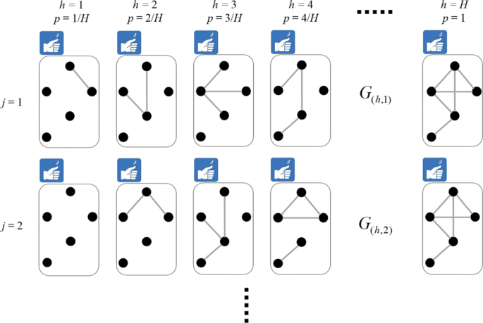

  

  Sampling algorithm

  Fig. 3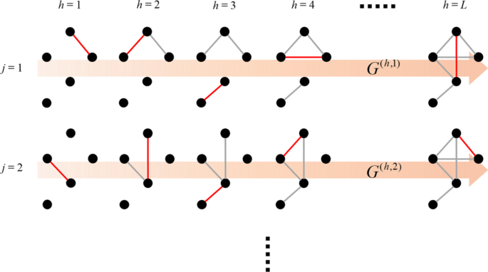

  

  Proposed sampling algorithm

  Fig. 4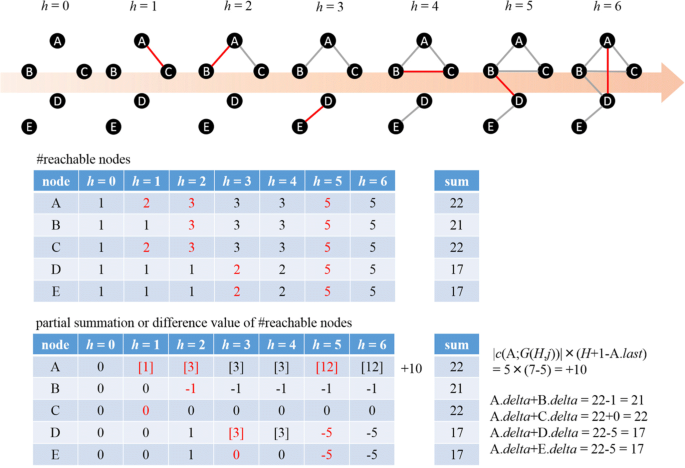

  

  Counting of reachable nodes

• We reformatted our proposed method and provide a pseudo code as Algorithms 1 and 2 to improve its understandability and readability.

• We prove that our proposed measures are unbiased estimators.

• We provide additional experimental results in “Results of connectedness centrality: cnc₃(v)” section and demonstrate how the proposed centrality is quite different from traditional centrality measures, specifically, closeness, betweenness, and eigenvector centrality, by comparing the top 1000 nodes identified in each centrality.

• We discussed how our proposed algorithm deals with non-uniform connection probabilities in “Extension: case of non-uniform connection probabilities” section and other types of networks in “Discussion” section.

• We also revised and extended our Introduction and Conclusion according to the above-mentioned additions.

The rest of our paper is organized as follows. In “Related work” section, we overview some related work and, in “Proposed measure” section, we explain in detail the proposed centrality measure and proposed algorithm. In “Experimental settings”, “Results of connectedness centrality: cnc₃(v)” and “Results of group connectedness centrality: $cnc_{3}(\mathcal {R})$” sections, we set forth and discuss the experimental settings and results. Furthermore, we discussed how our proposed algorithm deals with non-uniform connection probabilities and other types of networks in “Extension: case of non-uniform connection probabilities” section and “Discussion” section, and finally, we summarize our paper and propose future work in “Conclusion” section.

Related work

In this section, related work is organized from the viewpoint of centrality measure, community extraction, uncertain graphs, and facility location problems.

Centrality measure

In our method, each node is ranked by its connectedness score with neighbor nodes, which can be treated as a centrality measure. Some centrality measures for nodes have been proposed in sociology and web science, including degree, closeness, harmonic, betweenness, eigenvector, Katz, Bonacich, HITS, and PageRank (Freeman 1979; Katz 1953; Bonacich 1987; Brin and Page 1998; Kleinberg 1999). Since degree distribution does not follow power-law distribution and the maximum degree of nodes is relatively small due to geographical restrictions in road networks, degree centrality does not make sense. Closeness centrality and betweenness centrality take the shortest path between nodes into account, so these measures work well even in urban traffic networks, as reported in some studies (Crucitti et al. 2006; Park and Yilmaz 2010). Furthermore, eigenvector measures can extract subgraphs where high-degree nodes connect to each other. As a result, in a road network, it will be possible to extract urban districts where intersections with relatively high degrees are connected.

Our aim is to extract nodes with high connectedness scores, which can then be applied to candidate sites for evacuation facilities. When extracting such nodes, accessibility to these nodes can be an important factor. Closeness centrality quantifies accessibility based on distance, but does not take into consideration road blockages. Therefore, even if an extracted node is close to other nodes, if the node is located near a river, it is not a viable candidate location for an evacuation facility. Taken together, since some of the existing measures could extract important nodes in each of the notions for road networks, we experimentally compare the characteristics of related measures and ours.

Community extraction

Our method extracts representative nodes and divides the remaining nodes into clusters based on connectedness with the representative nodes, and thus can be treated as a community extraction method. In recent years, many methods for community extraction have been proposed (Seidman 1983; Girvan and Newman 2002; Clauset et al. 2004; Palla et al. 2005; von Luxburg 2007; Blondel et al. 2008; Chen and Hero 2015). However, these methods cannot straightforwardly apply to road networks, where the degrees of nodes roughly obey uniform distributions and there are little differences between the number of inter-community and intra-communities links. Furthermore, although spectral clustering (von Luxburg 2007) and deep community detection (Chen and Hero 2015) have a similar flavor to our method in terms of link cuttings, since the eigen-gaps of the Laplacian matrix and differences between the successive eigenvalues of spatial networks are quite small, unlike social networks, it is difficult to calculate the Fiedler vector of the Laplacian matrix with stability. This fact corresponds to the existence of some non-dominant communities and a few links that, when cut, isolate the spatial network. The Girvan-Newman (GN) method also cuts some links according to the edge-betweenness centrality and treats connected components of the remaining graph as communities (Girvan and Newman 2002). The GN method is based on a similar framework to our method in treating the connected components as communities by cutting edges; however, it is difficult to apply to large-scale networks due to its large computational complexity. Therefore, we compare our method with the CNM (Clauset, Newman, and Moore) method (Clauset et al. 2004), which directly optimizes the modularity function to accelerate the calculation and produces similar results to the GN method.

Uncertain graph

The uncertain graph has been studied within the broader context such as network reliability, querying, and mining. Jin et al. proposed two methods to efficiently and accurately estimate the probability that the distance between a given node pair of an uncertain graph is smaller than the designated value (Jin et al. 2011). In (Jin et al. 2011), the authors generalized the simple reachability problem to the distance-constraint reachability problem, which considers both distance and reachability in an uncertain graph. Therefore these methods can be useful in the context of evacuation activity. However, probability must be assigned to each link. Our method, on the other hand, integrates out all possibilities so that it does not need to preliminarily know the probability of each link. Our method adopts the deterministic recursive computational procedure in order to minimize the variance of the estimator and unequal probabilistic sampling over the enumeration tree in order to accelerate the sampling process.

Ceccarello et al. developed a node clustering method for an uncertain graph and reduced the treated problem to the k-center and k-median problems (Ceccarello et al. 2017). In this method, distances between nodes are defined by the inverse of the connection probability among them, which is efficiently and accurately estimated by the Monte Carlo sampling method. Potamias et al. introduced distance measures and identified the k-Nearest Neighbor nodes from an uncertain graph by calculating the probability of the distances between the arbitrary node pair based on the Monte Carlo sampling method with efficient pruning techniques in order to reduce the search space (Potamias et al. 2010). Pfeiffer et al. extended some structural indices on discrete graphs to probabilistic graphs by computing the expected values of sampling graph indices (Pfeiffer and Neville 2011).

Some research on stochastic graphs address another uncertainty. A stochastic graph is a fixed structure graph with randomly changing edge weights. The distribution of its change probability is unknown, but stationary. Misra et al. proposed a method that uses Learning Automata (LA) and Frigioni’s algorithm to find the statistical shortest path tree in an average graph topology for the dynamic single source shortest path problem (DSSSP) (Misra and Oommen 2005). Rezvanian et al. proposed generalization of some network measures for stochastic graphs using six LA-based algorithms to calculate these measures (Rezvanian and Meybodi 2016). Vahidipour et al. proposed an efficient LA-based algorithm that speeds up the process of finding the shortest path in a stochastic graph using parallelism for DSSSP (Vahidipour et al. 2017).

In contrast to these existing studies, which assume the connection strength as a probability value for each link, our method assumes a probability distribution for each link. Furthermore, our method also conducts Monte Carlo sampling and, as seen above, the efficiency and accuracy of these methods depend on the quality of the sampling techniques. Unlike the above-mentioned sampling methods, our proposed sampling algorithm is based on a time-evolving graph for which no link exists in a graph at the initial state and links are added to the graph one by one.

Facility location on graph

The most famous facility location problem is the k-median problem. The objective of the k-median problem is to minimize the sum of distances between citizens and their nearest facility, and many approximation algorithms have been reviewed (Alp et al. 2003; McKendall and Shang 2006; Levanova and Loresh 2004). As a facility location problem over graphs, a closeness-centrality-based method has been proposed (Tabata et al. 2017). Closeness centrality focuses on the graph distance and extracts the most central node with a minimum distance to the others. Although the method can quickly solve the location of a single facility, it cannot handle multiple facilities. Agra et al. (2017) provided a k-median problem algorithm for a graph that is divided into several connceted components like archipelagos. Since the approach assumes that it is known beforehand whether it is divided into connected components, it cannot deal with graph disruption by the stochastical occurrences of link breakages.

For locating evacuation facilities, the method proposed in (Kaveh et al. 2018) introduced a weight for each node that represents a risk factor like topographic conditions to the k-median problem. This method mainly considers the failure of nodes (facilities), but not the stochastic occurence of link disconnection. The method proposed by Puerto et al. considered the disruption possibility of an edge (Puerto et al. 2014), which has high computation costs. In fact, the only case of an efficient algorithm in the literature is k=1,2. Unlike these methods, our method attempts to extract multiple nodes as evacuation facility candidate sites based on connectedness with neighbor nodes calculated by an efficient and accurate sampling.

Proposed measure

In order to estimate node connectedness under a stochastic link disconnection, we propose a node ranking measure, called connectedness centrality, and its efficient sampling algorithm. To this end, we explain three versions of connectedness centrality measures. More specifically, we present the first centrality, called cnc₁, as a general theoretical framework and then derive the second, called cnc₂, as a computable measure by discretizing its prior probability distribution. We then propose a third, called cnc₃, as a practical measure equipped with its efficient estimation algorithm. This can be naturally explained as a special case of cnc₂, assuming that each link connection probability is the same, although this equal probability assumption can be easily relaxed, as shown in “Extension: case of non-uniform connection probabilities” section. Furthermore, to select multiple nodes, we propose group connectedness centrality by extending the target of connectedness centrality from each node to node groups.

Connectedness centrality: c n c ₁

Let $G = ({\mathcal {V}}, {\mathcal {E}})$ be the graph structure of a given spatial network. For each link $e \in {\mathcal {E}}$, we consider a link connection probability p(e;s) that is determined according to some model, such as a road blockage model, based on geographical properties, where s is a parameter, just like an inverse of magnitude of earthquake, to control the probability p(e;s). We set s in the range of 0≤s≤1 for our convenience. Figure 1 depicts an uncertain graph introducing connection probabilities to a given spatial network. For each link $e \in {\mathcal {E}}$, let x(e) be a random variable expressing the link connectivity, i.e., x(e)=1 if link e is connected; otherwise x(e)=0, where p(x(e)=1;s)=p(e;s). Then, by suitably arranging these random variables and setting $\Omega = \{0, 1\}^{|{\mathcal {E}}|}$, we can construct an indicator vector expressed as x=(⋯,x(e),⋯)∈Ω, whose total number of possible instantiations (possible worlds) amounts to $|\Omega | = |\{0, 1\}|^{|{\mathcal {E}}|} = 2^{|{\mathcal {E}}|}$. For each instance of the indicator vector x, we can obtain the corresponding graph $G_{\textbf {x}} = ({\mathcal {V}}, {\mathcal {E}}_{\textbf {x}})$, where ${\mathcal {E}}_{\textbf {x}}= \{e~|~e \in {\mathcal {E}}, x(e)=1\}$. In this paper, assuming a basic model based on independent Bernoulli trials for all links, with repect to each graph G_x obtained from x, we can compute its occurrence probability as follows:

$$ q(\mathbf{x}; s) = \prod_{e \in {\mathcal{E}}} p(e; s)^{x(e)} (1-p(e; s))^{1-x(e)} = \prod_{e \in {\mathcal{E}}_{\mathbf{x}}} p(e; s) \prod_{e \in {\mathcal{E}} \setminus {\mathcal{E}}_{\mathbf{x}}} (1-p(e; s)), $$

(1)

where ·∖· stands for a set difference operator. Here, we should emphasize that, unlike most studies on uncertain graphs, where each link connection probability is designated as a value, our approach specifies each as a stochastic model of link connection p(e;s) controlled by parameter s.

After decomposing G_x into connected components, we compute the size of each connected component as the number of nodes belonging to the component and let c(v;G_x) be the set of nodes belonging to the connected component in which node $v \in {\mathcal {V}}$ is included, where c(u;G_x)=c(v;G_x) if the nodes u and v belong to the same connected components. In this study, under a given stochastic model of link connection, we define our connectedness centrality of node $v \in {\mathcal {V}}$ by the expected size of the connected component where v is included. More specifically, for each node $v \in {\mathcal {V}}$, we quantify our first version of connectedness centrality by the following expectation:

$$ \phi_{1}(v) = cnc_{1}(v) = \int_{0}^{1} \sum_{\mathbf{x} \in \Omega} |c(v ;G_{\mathbf{x}})| q(\mathbf{x}; s) r_{1}(s) ds, $$

(2)

where r₁(s) stands for a prior probability distribution with respect to parameter s. For instance, it can be used to express the fact that small earthquakes occur frequently, but huge ones are quite rare.

Connectedness centrality: c n c ₂

Next, we consider computing the integration of s by the summation of H+1 equal interval points. Note that, for the h-th point (0≤h≤H), the link connection probability is set to p(e;h/H). Under this quantization, for each node $v \in {\mathcal {V}}$, we can quantify our second version of connectedness centrality by the following expectation:

$$ \phi_{2}(v) = \sum_{h=0}^{H} \sum_{\mathbf{x} \in \Omega} |c(v ;G_{\mathbf{x}})| q(\mathbf{x}; h) r_{2}(h), $$

(3)

where $r_{2}(h) = r_{1}(h/H)/\sum _{h'=0}^{H} r_{1}(h'/H)$.

Below, we propose computing the summation of $2^{|{\mathcal {E}}|}$ times by J Monte Carlo simulations. Let $G_{(h, j)} = ({\mathcal {V}}, {\mathcal {E}}_{(h, j)})$ be a graph obtained by the j-th simulation (1≤j≤J) at the h-th point (See Fig. 2); then, we can estimate our connectedness centrality ϕ₂(v) defined in Eq. (3) by the following:

$$ cnc_{2}(v) = \frac{1}{J} \sum_{h=0}^{H} \sum_{j=1}^{J} |c(v ;G_{(h, j)})| r_{2}(h). $$

(4)

Now, by considering the following expectation value of |c(v;G_x)| denoted by 〈|c(v;G_x)|〉_Ω, with respect to our simulation based on q(x;h/H),

$$ \langle |c(v ;G_{\mathbf{x}})| \rangle_{\Omega} = \sum_{\mathbf{x} \in \Omega} |c(v ;G_{\mathbf{x}})| q(\mathbf{x}; h/H), $$

(5)

we can see that cnc₂(v) is an unbiased estimator of ϕ₂(v), i.e.,

$$ \langle cnc_{2}(v) \rangle = \frac{1}{J} \sum_{h=1}^{H} \sum_{j=1}^{J} \langle |c(v ;G_{\mathbf{x}})| \rangle_{\Omega} r_{2}(h) = \phi_{2}(v). $$

(6)

Thus, by setting both H and J to sufficiently large values, we can naturally expect that cnc₂(v) defined in Eq. (4) can be reasonably accurately estimated to cnc₁(v) defined in Eq. (2). However, when straightforwardly computing cnc₂(v) for every $v \in {\mathcal {V}}$ for a large H and J, we need a large computational load because its computational complexity becomes O(HJ(N+L)), where $N = |{\mathcal {V}}|$ and $L = |{\mathcal {E}}|$ respectively stand for the numbers of nodes and links for a given network. Note that the computational complexity of decomposing a graph into its connected components is O(N+L) and, during this process, we can simultaneously compute their sizes.

Connectedness centrality: c n c ₃

Below, we propose another reasonably accurate estimate, referred to as cnc₃(v), instead of cnc₂(v) together with an effective algorithm whose computational complexity becomes O(J(L+N logN)), rather than O(HJ(N+L)). We assume that each link connection probability is the same, i.e., p(e;h/H)=p(h/H)=h/H, and define the set of graphs whose number of links is h, expressed as $\Omega (h) = \{ \mathbf {x}~|~\sum _{e \in {\mathcal {E}}} x(e) = h \}$. This definition corresponds to employing a setting of H=L. Under this uniform probability setting, for each node $v \in {\mathcal {V}}$, we can quantify our third version of connectedness centrality by the following expectation:

$$ \phi_{3}(v) = \sum_{h=0}^{H} \frac{1}{|\Omega(h)|} \sum_{\mathbf{x} \in \Omega(h)} |c(v ;G_{\mathbf{x}})| r_{2}(h). $$

(7)

Below, we estimate ϕ₃(v) by J Monte Carlo simulations.

In our proposed algorithm, from the initial state that all links are disconnected and thus all nodes are isolated in the setting p(0)=0, we repeatedly add a randomly selected link one by one until the final state where all original links are connected in the setting p(1)=1 (See Fig. 3). During this process, we attempt to efficiently compute the expected size of the connected component for each node $v \in {\mathcal {V}}$ by focusing on the difference between the graphs caused by adding only one link. More specifically, for the j-th simulation, we assign a random order to each link $e \in {\mathcal {E}}$, denoted by e^(h,j), where we also use h∈{1,⋯,H} to express the order that the link becomes connected. By considering a graph defined by $G^{(h, j)} = ({\mathcal {V}}, {\mathcal {E}}^{(h, j)})$, where ${\mathcal {E}}^{(h, j)} = \left \{ e^{(h', j)} \in {\mathcal {E}}~\left |~h' \leq h\right. \right \}$, we can estimate our connectedness centrality ϕ₃(v) defined in Eq. (7) by the following:

$$ cnc_{3}(v) = \frac{1}{J} \sum_{j=1}^{J} \sum_{h=1}^{H} \left|c\left(v ;G^{(h, j)}\right)\right| r_{2}(h). $$

(8)

By considering the following expectation value of |c(v;G_x)|, denoted by 〈|c(v;G_x)|〉_Ω(h), with respect to our simulation based on 1/|Ω(h)|,

$$ \langle |c(v ;G_{\mathbf{x}})| \rangle_{\Omega(h)} = \frac{1}{|\Omega(h)|} \sum_{\mathbf{x} \in \Omega(h)} |c(v ;G_{\mathbf{x}})|, $$

(9)

we can see that cnc₃(v) is an unbiased estimator of ϕ₃(v), i.e.,

$$ \langle cnc_{3}(v) \rangle = \frac{1}{J} \sum_{h=1}^{H} \sum_{j=1}^{J} \langle |c(v ;G_{\mathbf{x}})| \rangle_{\Omega(h)} r_{2}(h) = \phi_{3}(v). $$

(10)

Thus, for uniform probability settings, by setting both H and J to sufficiently large values, we can naturally expect that cnc₃(v) defined in Eq. (8) can be a reasonably accurate estimate of cnc₁(v) defined in Eq. (2).

Solution algorithm of c n c ₃

Below, we provide details of our proposed algorithm together with its computational complexity. In the initial state with no link, we set that every node belongs to an individually different component by assigning a unique component number n(v)∈{1,⋯,N} to each node $v \in {\mathcal {V}}$. When a new link (represented by a red link in Fig. 3) denoted by e^(h,j)=(x,y)^(h,j) is added, we can proceed to the next link if nodes x and y belong to the same connected component; otherwise, we need to change the component number of nodes belonging to one component.

More specifically, by assuming |c(x;G^(h,j))|≥|c(y;G^(h,j))| without loss of generality, we propose that the component number with a smaller size is changed to a larger one by setting n(z)←n(x) for each z∈c(y;G^(h,j)). Evidently, for each link addition, the number of nodes whose component number is changed never exceeds N/2. Thus, during all link additions, the computational complexity of these renumbering processes becomes O(N logN).

Let $cnc_{3}^{(h, j)}(v)$ be the partial summation of $\left |c\left (v ;G^{(h', j)}\right)\right |\phantom {\dot {i}\!}$ until h^′=h for the j-th simulation defined by

$$ cnc_{3}^{(h, j)}(v) = \sum_{h'=1}^{h} \left|c\left(v ;G^{(h', j)}\right)\right| r_{2}(h'). $$

(11)

Now, suppose that when a new link e^(h,j)=(x,y)^(h,j) was added at the h-th step, nodes x and y switch to belong to the same connected component for the first time. For arbitrary h^′≥h, since $\phantom {\dot {i}\!}c\left (x ;G^{(h', j)}\right) = c\left (y ;G^{(h', j)}\right)$, we can obtain the following relation:

$$ cnc_{3}^{(h', j)}(x) - cnc_{3}^{(h', j)}(y) = cnc_{3}^{(h-1, j)}(x) - cnc_{3}^{(h-1, j)}(y). $$

(12)

Thus, by maintaining the partial summation $cnc_{3}^{(h', j)}(x)$ for a head node x of each connected component and keeping the difference values such as $cnc_{3}^{(h-1, j)}(x) - cnc_{3}^{(h-1, j)}(y)$ for the other nodes in the component, we can obtain the final summation values, such as $cnc_{3}^{(H, j)}(y)$, by using Eq. (12). Note that the computational complexity of obtaining $cnc_{3}^{(h, j)}(v)$ for every $v \in {\mathcal {V}}$ is O(N) and that of updating these difference values is O(N logN) because these updates can be done together with the above node renumbering processes. Therefore, since we need to shuffle and examine all of the links at the j-th simulation, the total computational complexity of our proposed algorithm becomes O(J(L+N logN)). Algorithm 1 and Fig. 4 show the details of the algorithm of connectedness centrality. In Algorithm 1, delta has two meanings: for the head node s of a connected component at step h, s.delta indicates the partial sum of reachable nodes $cnc_{3}^{(h-1,j)}(s)$; for the other appearing node x, x.delta indicates the difference value of the partial summation of the reachable nodes between node x and its head node s, $cnc_{3}^{(h,j)}(x)-cnc_{3}^{(h,j)}(s)$.

Group connectedness centrality

Although we can extract high-connectedness nodes using our connectedness centrality, these nodes gather unevenly in some parts of the network because of focusing on whether or not they belong to the large connected component. Actually, as shown in “Results of connectedness centrality: cnc₃(v)” section, the top 1000 nodes of the connectedness centrality ranking are located near each other. This tendency is impractical for the purpose of estimating evacuation facility locations. To overcome this shortcoming, we enhance the notion of our connectedness centrality, called group connectedness centrality.

In group connectedness centrality, connectedness of the node set ${\mathcal {R}}$ is defined as:

$$ cnc_{1}({\mathcal{R}}) = \int_{0}^{1} \sum_{\mathbf{x} \in \{0, 1\}^{|{\mathcal{E}}|}} |c({\mathcal{R}} ;G_{\mathbf{x}})| q(\mathbf{x}; s) r_{1}(s) ds, $$

(13)

where $c({\mathcal {R}} ;G_{\mathbf {x}}) = \bigcup _{r \in {\mathcal {R}}}c(r ;G_{\mathbf {x}})$ stands for the number of reachable nodes from whichever of $r \in {\mathcal {R}}$.

Similarly to connectedness centrality, we compute the integration of s by the summation of H+1 equal interval points and set r(s) to be a uniform distribution.

$$ cnc_{3}({\mathcal{R}}) = \frac{1}{J} \sum_{j=1}^{J} \sum_{h=1}^{H} \left|c\left({\mathcal{R}} ;G^{(h, j)}\right)\right| r_{2}(h). $$

(14)

In order to select K nodes, ${\mathcal {R}}$, which maximizes the objective function defined in Eq. (14), we utilize a greedy algorithm. Hereafter, we refer to the selected node as the representative node. When selecting k-th representative node ${\hat r}_{k}$, the greedy algorithm fixes k−1 already selected nodes ${\mathcal {R}}_{k-1}$ and selects the node with the highest marginal gain, MG, defined by

$$\begin{array}{@{}rcl@{}} MG(v; {\mathcal{R}}_{k-1}) &=& cnc_{3}({\mathcal{R}}_{k-1} \cup \{v\}) - cnc_{3}({\mathcal{R}}_{k-1}) \\ &=& \frac{1}{J} \sum_{j=1}^{J} \sum_{h=1}^{H} mg(v;{\mathcal{R}}_{k-1})^{(h, j)} r_{2}(h), \end{array} $$

(15)

where $mg(v;{\mathcal {R}}_{k-1})^{(h, j)} = \left |c\left ({\mathcal {R}}_{k-1} \cup \{v\} ;G^{(h, j)}\right) \setminus c\left ({\mathcal {R}}_{k-1} ;G^{(h, j)}\right)\right |$ stands for the increment of the number of reachable nodes when node v, which is a candidate for the k-th representative node, is added to ${\mathcal {R}}_{k-1}$. The total computational complexity of group connectedness centrality becomes O(KJ(L+N logN)). Let ${\mathcal {Q}}$ be a subset of ${\mathcal {R}}$, i.e., ${\mathcal {Q}} \subset {\mathcal {R}}$. Then we obtain $mg(v;{\mathcal {Q}})^{(h,j)} \geq mg(v;{\mathcal {R}})^{(h,j)}$, which directly derives $MG(v;{\mathcal {Q}}) \geq MG(v;{\mathcal {R}})$ from the definition of $MG(v;{\mathcal {R}})$ shown in Eq. (15). Therefore, we can see that $cnc_{3}({\mathcal {R}}))$ is a submodular function, and thus its greedy solution guarantees to be reasonably high quality with the worst case.

After selecting K representative nodes, each of the remaining nodes is assigned to the community where a representative node with the highest connectedness exists. Suppose that when a new link is added at the h-th step of the j-th simulation, node v switches to belong to the same connected component with representative node r. The degree of connectedness of nodes v and r is then defined as f(v,r)^(j)=1−h/H. Therefore, the degree of connectedness in all J simulations is $F(v, r) = J^{-1}\sum _{j = 1}^{J} f(v, r)^{(j)}$. For each of the remaining nodes, we assign one community of a representative node with the highest connectedness as follows:

$${\mathcal{V}}^{(k)} = \{v \in {\mathcal{V}}; r_{k} = \text{arg~max}_{r \in {\mathcal{R}}} F(v,r) \}. $$

In the final stage of a simulation, when most representative nodes would belong to the same connected component and the degree of connectedness between a remaining node v and each representative node is equal, node v is assigned to the community of the closest representative node in terms of graph distance. Hereafter, we refer to this method as CNC and show the summary of CNC in Algorithm 2.

In the context of the evacuation facility location problem, the representative node corresponds to a candidate site for an evacuation facility.

Experimental settings

To reveal the characteristics of our method, we conducted several experiments using actual datasets to compare our method with some existing methods.

Dataset

In our experiments, we employed the following four prefectures extracted from Digital Road Map (DRM) data: Tokyo, Kanagawa, Shizuoka, and Ibaraki. We extracted all intersections and roads from the DRM data of each prefecture. We then constructed a spatial network with the intersections as the nodes and the roads between the intersections as the links by following a standard formulation of road networks such as those presented by SNAP (Stanford Large Network Dataset Collection)¹. Namely, we deleted nodes used for the curve-segments of roads by directly connecting intersections at both ends of these curve-segments, where the curve-segment nodes mean points representing polylines between intersections in DRM, which are used to approximate the road shapes. As a result, each network has 340919, 295151, 110925, and 172892 nodes, and 485858, 402576, 162322, and 263075 links, respectively.

Existing methods used for comparison

We used the following three centrality measures and two clustering (community extraction) methods for comparison. We begin by briefly discussing the centrality:

• Closeness centrality

  Closeness centrality is calculated based on the average of the shortest path length d(u,v) between pairs of nodes. In this paper, we employed a harmonic version using the inverse value of the distance.

  $$clc(v) = \sum_{u \in {\mathcal{V}} \setminus \{v\}} d(v,u)^{-1} $$

• Betweenness centrality

  Betweenness centrality is calculated based on the number of shortest paths between any pair of nodes.

  $$bwc(v) = \sum_{s \in {\mathcal{V}} \setminus \{v\}} \sum_{t \in {\mathcal{V}} \setminus \{s,v\}} \frac{\sigma_{s,t}(v)}{\sigma_{s,t}}, $$

  where σ_s,t is the number of shortest paths between s and t, and σ_s,t(v) is the number of routes going through v of them.

• Eigenvector centrality

  Eigenvector centrality is based on the dominant eigenvector of the adjacency matrix and calculated using the power iteration method.

  $$eig_{t+1}(v) = \sum_{u \in \Gamma(v)} eig_{t}(u),~~eig_{t+1}(v) \gets \frac{eig_{t+1}(v)}{\sum_{u \in {\mathcal{V}}} eig_{t+1}^{2}(u)}, $$

  where Γ(v) is the set of adjacent nodes of v. We used the converged value eig_t(v) as centrality score eig(v).

Next, we show the abstract of the community extraction methods:

• Distance-based method

  We extend the closeness centrality to group closeness centrality similarly to our group connectedness centrality.

  $$ clc({\mathcal{R}}) = \sum_{v \in {\mathcal{V}}} \max_{r \in {\mathcal{R}}} d(v,r)^{-1}. $$

  (16)

  To maximize the objective function Eq. (16), we employ a greedy algorithm as well as our group closeness centrality. Extracting a node set ${\mathcal {R}}$ consisting of K representatives and assigning each of the remaining nodes to a community based on the shortest path length to the representative node is equivalent to conducting K-medoids clustering based on the graph distance. Hereafter, we refer to this method as CLC.

• Density-based method

  In this study, we employed a well-known community extraction method, the CNM method (Clauset et al. 2004), which directly optimizes the modularity function to accelerate the calculation. The CNM method divides all nodes into K communities without extracting representative nodes. Therefore, just for reference, we utilize the CNM method as a general community extraction method.

Results of connectedness centrality: c n c ₃(v)

How to determine parameter J?

We first experimentally examine the quality of the connectedness centrality calculations. The value of cnc₃(v) depends on the parameter, which is the number of simulations J. As mentioned above, when increasing the number of simulations J, the expected value of cnc₃(v) approaches the true value because cnc₃(v) is the unbiased estimator. To confirm the variance of cnc₃(v) with respect to J, we conducted M calculations and introduced the coefficient of variation, $CV(v) = \sigma (v)/\overline {cnc}_{3}(v)$, where $\overline {cnc}_{3}(v) = M^{-1}\sum _{m=1}^{M} cnc_{3}(v;m)$ stands for the arithmetic mean of the value by the m-th calculation, cnc₃(v;m), 1≤m≤M, and $\sigma (v) = M^{-1}\sum _{m=1}^{M} (cnc_{3}(v;m)-\overline {cnc}_{3}(v))^{2}$ is a sample standard deviation. Figure 5 shows the coefficient of variation for M=100 calculations, where the horizontal axis is the connectedness centrality score cnc₃(v). In each of the calculations, we set the number of simulations to J=10000.

Fig. 5

Coefficient of variation

From Fig. 5, we can confirm that, for all networks, the value of CV(v) is significantly small, especially for the nodes with high scores. Moreover, generally speaking, the value of CV(v) becomes $1/\sqrt {J}$ with respect to the increase of J. Based on the results of this verification, in the remainder of this paper, the result of J=10000 will be shown unless otherwise noted.

Comparison with other centrality measures

We now compare the top nodes in the ranking of existing centrality measures that can be naturally applied to road networks and proposed connectedness centrality. Let CENT(r) and PROP(r) be the node set up to the upper r ranking of the existing and the proposed centrality, and quantitatively investigate the ranking similarity using the F-measure (Rijsbergen 1979) defined as follows:

$$F(r) = \frac{2 \cdot |PROP(r) \cap CENT(r)|}{|PROP(r)|+|CENT(r)|}. $$

Figure 6 shows the F-measure with respect to the ranking. Figure 6 shows that, in the four networks, the F-measure is almost 0 up to the top 1000 and thus the rankings do not almost match; that is, different nodes are extracted as important nodes by each centrality.

Fig. 6

Similarity of centrality rankings

Figure 7 plots the top 1000 nodes in the proposed and existing centrality rankings in the Shizuoka network. The highly ranked nodes of the connectedness centrality are distributed in wide plain areas, especially residential areas. In the residential area in the plain part, since there are many routes to other nodes and some routes are blocked, alternative routes can be used. Thus, the connectedness of these nodes with neighbors is high. Nodes on important roads such as expressways are selected as highly ranked nodes of the closeness and betweenness centralities. While high-closeness nodes are chosen from the central region of the network, high-betweenness nodes are chosen from the entire network. Highly eigenvector-centrality-ranked nodes are selected from the downtown area around a station. Although not shown, in the ranking based on the second eigenvector, the nodes of the downtown area around the other station were extracted. In this way, various centrality measures can extract important nodes from the road network, but their meanings are significantly different.

Fig. 7

Top 1000 nodes of centrality rankings (Shizuoka network). a Connectedness centrality. b Closeness centrality. c Betweenness centrality. d Eigenvector centrality

Results of group connectedness centrality: $cnc_{3}(\mathcal {R})$

In this section, we evaluate the group connectedness centrality from the viewpoints of stability with respect to the number of simulations, reachability to the extracted representative nodes, and computation time. In our experimental scenario, we set the number of representatives (evacuation facilities) K as a relatively small number, like K=5,10,15,20, because, in practical terms, installation cost should be considered and the number of facilities that can be installed in each municipality is restricted.

Stability with respect to the number of simulations

In this subsection, we show the stability of group connectedness centrality with respect to the number of simulations J. In this experiment, we conducted CNC calculation 10 times while changing the number of simulations J=10¹,10²,10³,10⁴. We regard a result with J=100,000 as converged and compare the results in terms of similarities of representative nodes and communities. Figure 8a depicts the Minimum Matching Distance (MMD) between representatives extracted by each CNC computation, which is calculated as follows:

$$MMD(J) = \frac{1}{K} \sum_{k=1}^{K} \min_{1 \leq h \leq K} e(r(k), r(h;J)) +\frac{1}{K} \sum_{k=1}^{K} \min_{1 \leq h \leq K} e(r(k;J), r(h)), $$

where r(k) and r(k,J) respectively stand for the k-th representative node extracted by a CNC computation with 100,000 and J simulations, and e(a,b) is the Euclidean distance between locations of two representatives a and b. In Fig. 8a, the red solid line is the mean of MMD(J) at 10 times with respect to the number of simulations J taken as the horizontal axis and the black lines stand for the average Euclidean distances between node pairs of $\Gamma _{d} = \{(u, v) \in {\mathcal {V}} \times {\mathcal {V}}; d(u,v) = d\},~~d=1,5,10$. As illustrated by Fig. 8a, the average MMD decreases as the number of simulations J increases and, especially at J=10⁴, indicates about the same or less value than the average distance of Γ₅. This means that almost the same representatives are extracted.

Fig. 8

Stability w.r.t. the number of simulations (K=20). a Similarity between representatives. b Similarity between communities

Figure 8b depicts the Normalized Mutual Information (NMI) between communities assigned to the nodes by each CNC computation. From Fig. 8b, the average NMI takes a substantially large value, i.e., NMI(J)≃0.9, which means that almost the same communities are extracted. These results confirm that stable results can be obtained with a substantially small number of simulations compared with the number of possible worlds J≪2^L. Although we show the results with setting K=20, which is the largest in our settings, similar results were obtained with K=5,10,and15.

Visualization of representatives and their communities

Next, we qualitatively evaluate our method, CNC, compared with two existing methods, CLC and CNM, by visualizing the extracted communities shown in Fig. 9b, c, and d. Due to the limitation of the number of pages, we show only the results of the Shizuoka network with setting K=20, which is the largest of our experiments, but similar results were obtained in other networks with settings K=5,10,and15. In Fig. 9b and c, the representative nodes are described as star nodes and the colors of other nodes stand for their assigned communities. Figure 9a depicts the natural environment in and around the Shizuoka network, such as mountains and rivers, which can be constraints during evacuations. Figure 9b shows that our CNC method extracts representatives (star nodes) avoiding mountainous areas and divides nodes into communities roughly according to the natural environment. For some representatives (surrounded by circles in Fig. 9b), although they are located in lakeside, streamside, and peninsula areas and are easily isolated, many nodes exist around them. Therefore, evacuation facilities are needed in these areas. On the other hand, in the CLC and the CNM methods’ results, several communities (surrounded by squares in Fig. 9c and d) range across rivers and mountains. In Fig. 9c, two circled representative nodes are located in the mountainous areas; thus access to the residents of these communities may be difficult during disasters.

Fig. 9

Visualization of Shizuoka network (K=20). a Landmarks. b CNC. c CLC. d CNM

Reachability under link cutting

In this subsection, we quantitatively evaluate the reachability of the extracted representative nodes under a link disconnection situation, which models road blockage. In this experiment, we remove a certain ratio of links according to edge-betweenness centrality or random-selection. We then examine whether the representative node can be reached from the non-representative nodes along with existence links.

First, we count the number of reachable representative nodes from each non-representative node where a certain ratio of high edge-betweenness links is removed. Figure 10 shows the average number of reachable representatives with respect to the cutting rate taken as the horizontal axis. From Fig. 10, for all networks and all communities, K, the average number of reachable representatives extracted by our CNC method is substantially larger than those by the CLC method. In particular, even though 10% of the links are removed, at least one representative node can be reached from non-representative nodes for any number of representatives. Although, as the number of representative nodes increases, the difference between the results of the two methods tends to gradually decrease, the proposed method is sufficient with a smaller number of representative nodes for obtaining the same degree of reachability to the representatives extracted by CLC. For example, if setting up K=5 evacuation facilities for the Tokyo network, each resident can reach two to five proposed evacuation sites on average (red line in the left top image of Fig. 10a). In order to achieve the same degree of reachability, 15 evacuation facilities are required (green line in the left bottom image of Fig. 10a).

Fig. 10

Reachability of the representatives under high-betweenness-link cutting. a tokyo. b kanagawa. c shizuoka. d ibaraki

Next, we show the average number of nodes reachable to representatives within a certain distance d in Fig. 11, where the dotted and solid lines indicate the distances d=10 and d=20, respectively. In almost all the graphs of Fig. 11, we see that 1) when the cutting probability is 0, that is, when the graph is not disconnected, many more nodes can reach the representatives extracted by CLC than CNC; 2) as the cutting probability increases, more nodes reach the representatives extracted by CNC than CLC. Although the CLC method can extract nodes with the smallest sum of distances in situations where the graph is not disconnected, we confirmed that many nodes cannot be reached if the graph becomes disconnected.

Fig. 11

Distance to the representatives under high-betweenness-link cutting. a tokyo. b kanagawa. c shizuoka. d ibaraki

Similarly to the results shown in Fig. 10, we removed a certain ratio of links selected uniformly at random and examined whether the representative node can be reached from the non-representative nodes along with existence links (Fig. 12a). In the experiment, we executed link removal trials 10 times and calculated the average number of reachable nodes. Unlike the results in Fig. 10, the difference between the two methods is substantially small in any network. Similarly to Figs. 11, 12b shows the average number of nodes reachable to representatives within a certain distance d. Unlike the results in Fig. 11, more nodes can reach the CLC representatives; however, the number of nodes that can reach the CNC representatives is almost the same as that of high-betweenness-link cutting. Therefore, the CNC method can stably extract promising representative nodes robust to both types of link cuttings. Although not shown, similar results were obtained for the other networks.

Fig. 12

Reachability and distance of the representatives under random-link cutting (Tokyo). a Reachability. b Distance

From these results, in the context of the evacuation facility problem, residents can be expected to reach evacuation facilities extracted by our method even when blockages of high-betweenness roads like a bridge between cities occur.

Computation time

Finally, we evaluate our method from the viewpoint of computation time. Figure 13a and b show the computation time with respect to the number of simulations J and communities K, respectively. As might be expected, Fig. 13a shows that, when the number of simulations J increases, computation time increases; however, even at J=10000, CNC is faster than CLC. Moreover, Fig. 13b shows that the difference between the computation time of the CNC and CLC methods increases as the number of communities K grows. Therefore, our method can output a number of representative nodes and their communities more efficiently even for large-scale networks.

Fig. 13

Computation time. a w.r.t. #simulations J (K=10). b w.r.t. #communities K (J=10000)

Extension: case of non-uniform connection probabilities

Although our proposed cnc₃ algorithm was derived by assuming the case of the uniform connection probability for all links, it should be mentioned that, by adequately transforming a given simple graph into a multigraph and/or by adequately introducing some virtual nodes and links, we can easily deal with the case of non-uniform ones even with our current algorithm. Our algorithm is straightforwardly applicable to a multigraph. More specifically, we denote the multiplicity of a link $e \in {\mathcal {E}}$ by m(e) and let e and f be links whose multiplicities are m(e)=1 and m(f)=2, respectively, which means that a multiset {e,f,f} is a subset of ${\mathcal {E}}$, that is, $\{e, f, f\} \subset {\mathcal {E}}$. Then, for a list of links produced by randomly arranging each element in ${\mathcal {E}}$, the probability that at least one f appears prior to e is twice the probability that e appears prior to both of them, indicating that we can naturally implement a non-uniform probability, p(f;s)=2p(e;s), since the second occurrence of f is simply ignored in terms of connectedness. This suggests that, by adequately transforming a given simple graph into a multigraph, we can easily deal with the case of non-uniform probabilities.

As another way to deal with the case of non-uniform probabilities, we can consider adding virtual nodes and links. More specifically, let (u,v) and (w,x) be links in a simple graph $G({\mathcal {V}}, {\mathcal {E}})$. After removing (u,v), we add two links (u,y) and (y,v) by introducing a completely new node $y \not \in {\mathcal {V}}$, which produces a new graph $G'({\mathcal {V}}', {\mathcal {E}}')$ where ${\mathcal {V}}' = {\mathcal {V}} \cup \{y\}$ and ${\mathcal {E}}' = ({\mathcal {E}}\setminus \{(u,v)\}) \cup \{(u,y), (y,v)\}$. From our uniform setting, we obtain p((u,y);s)=p((y,v);s)=p((w,x);s) for G^′. Then, for a list of links produced by randomly arranging each element in ${\mathcal {E}}'$, the probability that both (u,y) and (y,v) appear prior to (w,x) is half the probability that e appears prior to one of them, indicating that we can also naturally implement a non-uniform probability, p((u,v);s)=0.5p((w,x);s), over the original graph G. This suggests that, by adequately introducing some virtual nodes and links, we can easily deal with the case of non-uniform probabilities. In this paper, although our algorithm deals with the case of non-uniform probabilities over a multigraph as mentioned above, to evaluate the basic performance of our proposed algorithm, we focus only on the case of uniform probability over a simple graph.

Discussion

Our problem setting is very closely related to percolation problems and introducing the percolation states of individual nodes into our problem formulation is an interesting research direction, as performed in the percolation centrality proposed by Piraveenan et al. (2013). In addition, since our proposed algorithm is quite efficient and works linearly with the problem size for each simulation, as another research direction, we expect that our method can more efficienctly solve some percolation problems.

On the other hand, our proposed algorithm can contribute to some types of dynamic networks analyses. In fact, as to some sort of dynamic networks that incrementally evolve by addition of a link over time, we can directly apply our algorithm for efficiently computing the average number of reachable nodes with respect to every node in a dynamic network during a given period. Moreover, since it is straightforward to enable to cope with the deletion of a link, our algorithm is expected to be served as a basic tool for this type of reachability analyses, although we need to confirm the validity of this claim by performing further experiments in future.

In addition to the above future directions, our immediate future work includes evaluating both the effectiveness of our connectedness centrality and the efficiency of our algorithm for the other types of networks such as social networks with non-uniform connection probabilities. For this purpose, in order to clarify the basic characteristics of our centrality and algorithm, we plan to utilize representative synthetic networks produced by Erdos-Renyi, Barabasi-Albert, and stochastic block models. Furthermore, our method, in particular, the objective function and its marginal gain on the CNC method, could quantitatively evaluate existing facilities from the viewpoints of reachability to each facility, contribution of each facility and its duplication degree which helps planning not only of the new construction but also of the abolishment. Therefore, it can be expected that more effective evacuation facility installation would be realized by objectively quantifying the degree of contribution of some candidate sites devised by domain experts using our objective function.

Conclusion

In this paper, to extract high-connectedness nodes from large-scale networks, we proposed connectedness centrality and its extended version, group connectedness centrality, together with an efficient sampling method based on a time-evolving graph. The proposed method can be regarded as a generalization of connected component decomposition intended for a connected graph. In experiments using actual road networks, we confirmed that 1) connectedness centrality can quantify the degree of connectedness with neighboring nodes and extract high-connectedness nodes; and 2) group connectedness centrality can extract adequate representative nodes from the viewpoints of their location, community members, and reachability. We further confirmed that our approximation based on sampling technique is efficient and effective in terms of computation time and stability with respect to the number of simulations.

As future work, we plan to develop an extended version of connectedness centrality that takes non-uniform values as link connection probabilities into account and confirm whether our method can apply to more varied types of networks.

References

Agra, A, Cerdeira JO, Requejo C (2017) A decomposition approach for the p-median problem on disconnected graphs. Comput Oper Res 86:79–85.
Alp, O, Erkut E, Drezner Z (2003) An efficient genetic algorithm for the p-median problem. Ann Oper Res 122:21–42.
Blondel, VD, Guillaume JL, Lambiotte R, Lefebvre E (2008) Fast unfolding of communities in large networks. J Stat Mech Theory Exp 2008(10):P10,008.
Bonacich, P (1987) Power and Centrality: A Family of Measures. Am J Sociol 92(5):1170–1182. https://doi.org/10.2307/2780000.
Brin, S, Page L (1998) The anatomy of a large-scale hypertextual web search engine. Comput Netw ISDN Syst 30:107–117.
Ceccarello, M, Fantozzi C, Pietracaprina A, Pucci G, Vandin F (2017) Clustering uncertain graphs. Proc VLDB Endowment 11(4):472–484.
Chen, PY, Hero AO (2015) Deep community detection. IEEE Trans Signal Process 63(21):5706–5719.
Clauset, A, Newman MEJ, Moore C (2004) Finding community structure in very large networks. Phys Rev E 70(6):066,111+. https://doi.org/10.1103/PhysRevE.70.066111.
Crucitti, P, Latora V, Porta S (2006) Centrality Measures in Spatial Networks of Urban Streets. Phys Rev E 73(3):036,125+.
Freeman, L (1979) Centrality in social networks: Conceptual clarification. Soc Netw 1(3):215–239. https://doi.org/10.1016/0378-8733(78)90021-7.
Fushimi, T, Saito K, Ikeda T, Kazama K (2018) A New Group Centrality Measure for Maximizing the Connectedness of Network Under Uncertain Connectivity In: Proceedings of the 7th International Conference on Complex Networks and Their Applications, 3–14.. Springer.
Girvan, M, Newman MEJ (2002) Community structure in social and biological networks. Proc Natl Acad Sci 99(12):7821–7826. https://doi.org/10.1073/pnas.122653799.
Jin, R, Liu L, Ding B, Wang H (2011) Distance-constraint reachability computation in uncertain graphs. Proc VLDB Endowment 4(9):551–562.
Katz, L (1953) A new status index derived from sociometric analysis. Psychometrika 18:39–43.
Kaveh, A, Beitollahi A, Mahdavi V (2018) Locating emergency facilities using the weighted k-median problem: A graph-metaheuristic approach. Period Polytech Civ Eng 62(1):200–205.
Kleinberg, JM (1999) Authoritative sources in a hyperlinked environment. J ACM 46:604–632.
Levanova, TV, Loresh MA (2004) Algorithms of ant system and simulated annealing for the p-median problem. Autom Remote Control 65(3):431–438.
von Luxburg, U (2007) A tutorial on spectral clustering. Stat Comput 17(4):395–416.
McKendall, AR, Shang J (2006) Hybrid ant systems for the dynamic facility layout problem. Comput Oper Res 33(3):790–803.
Misra, S, Oommen BJ (2005) Dynamic algorithms for the shortest path routing problem: learning automata-based solutions. IEEE Trans Syst Man Cybern Part B (Cybern) 35(6):1179–1192.
Palla, G, Derényi I, Farkas I, Vicsek T (2005) Uncovering the Overlapping Community Structure of Complex Networks in Nature and Society. Nature 435:814–818.
Park, K, Yilmaz A (2010) A Social Network Analysis Approach to Analyze Road Networks In: Proceedings of the ASPRS Annual Conference 2010.
Pfeiffer, JJ, Neville J (2011) Methods to determine node centrality and clustering in graphs with uncertain structure In: Proceedings of the Fifth International Conference on Weblogs and Social Media, 590–593.. The AAAI Press.
Piraveenan, M, Prokopenko M, Hossain L (2013) Percolation centrality: Quantifying graph-theoretic impact of nodes during percolation in networks. PLoS ONE 8(1):e53,095. https://doi.org/10.1371/journal.pone.0053095.
Potamias, M, Bonchi F, Gionis A, Kollios G (2010) K-nearest neighbors in uncertain graphs. Proc VLDB Endowment 3(1-2):997–1008.
Puerto, J, Ricca F, Scozzari A (2014) Unreliable point facility location problems on networks. Discret Appl Math 166:188–203.
Rezvanian, A, Meybodi MR (2016) Stochastic graph as a model for social networks. Comput Hum Behav 64(C):621–640.
Rijsbergen, CJV (1979) Information Retrieval, 2nd edn.. Butterworth-Heinemann, Newton.
Seidman, SB (1983) Network structure and minimum degree. Soc Netw 5(3):269–287.
Tabata, K, Nakamura A, Kudo M (2017) An efficient approximate algorithm for the 1-median problem on a graph. IEICE Trans Inf Syst E100.D(5):994–1002. https://doi.org/10.1587/transinf.2016EDP7398.
Vahidipour, SM, Meybodi MR, Esnaashari M (2017) Finding the shortest path in stochastic graphs using learning automata and adaptive stochastic petri nets. Int J Uncertain Fuzziness Knowl-Based Syst 25(3):427–455.
Acknowledgments
We thank Prof. Seiya Okubo of the University of Shizuoka, Shizuoka, Japan, for supporting computation environments.
Funding
All authors are grateful for the financial support from JSPS Grant-in-Aid for Scientific Research (No.17H01826).
Author information
Authors and Affiliations
Contributions
TF performed the research and wrote the article. KS contributed to designing the proposed method. TI contributed preparation of experimental data and part of experimental evaluations. KK contributed survey of related work and part of experimental evaluations. All authors read and approved the final manuscript.
Corresponding author
Ethics declarations
Competing interests
All authors declare no financial and non-financial competing interests.
Additional information
Publisher’s Note
Springer Nature remains neutral with regard to jurisdictional claims in published maps and institutional affiliations.
Rights and permissions
Open Access This article is distributed under the terms of the Creative Commons Attribution 4.0 International License(http://creativecommons.org/licenses/by/4.0/), which permits unrestricted use, distribution, and reproduction in any medium, provided you give appropriate credit to the original author(s) and the source, provide a link to the Creative Commons license, and indicate if changes were made.
About this article
Cite this article
Fushimi, T., Saito, K., Ikeda, T. et al. Estimating node connectedness in spatial network under stochastic link disconnection based on efficient sampling. Appl Netw Sci 4, 66 (2019). https://doi.org/10.1007/s41109-019-0187-3
Received:
Accepted:
Published:
DOI: https://doi.org/10.1007/s41109-019-0187-3