- Research
- Open access
- Published:
Error-correcting decoders for communities in networks
Applied Network Science volume 4, Article number: 9 (2019)
Abstract
As recent work demonstrated, the task of identifying communities in networks can be considered analogous to the classical problem of decoding messages transmitted along a noisy channel. We leverage this analogy to develop a community detection method directly inspired by a standard and widely-used decoding technique. We further simplify the algorithm to reduce the time complexity from quadratic to linear. We test the performance of the original and reduced versions of the algorithm on artificial benchmarks with pre-imposed community structure, and on real networks with annotated community structure. Results of our systematic analysis indicate that the proposed techniques are able to provide satisfactory results.
Introduction
Real networks often exhibit organization in communities, intuitively defined as groups of nodes with a higher density of edges within rather than between groups (Girvan and Newman 2002; Fortunato 2010). Most of the research on this topic has focused on the development of algorithms for community identification. Proposed approaches vary widely, including hierarchical clustering algorithms (Friedman et al. 2001), modularity-based methods (Newman and Girvan 2004; Newman 2004; Clauset et al. 2004; Guimera et al. 2007; Duch and Arenas 2005; Newman ME 2006a; Newman ME 2006b), random walk based algorithms (Zhou 2003; Rosvall and Bergstrom 2008), and statistical inference methods (Newman and Leicht 2007; Hastings 2006; Decelle et al. 2011b; Karrer and Newman 2011; Peixoto 2014; 2013; 2018), to mention a few of them. Whereas algorithms differ much in spirit, they all share two intrinsic limitations. First, as described by the No Free Lunch Theorem (Peel et al. 2017), there is no community detection algorithm that works best for all networks and community structures; an algorithm good for one class of networks may be equally bad for another class of networks. A second type of limitation arises from self-consistency tests, where community detection methods are applied to instances of the stochastic block model to uncover the community structure pre-imposed in the model. Algorithms can recover a non-vanishing portion of the true community structure of the graph only if the amount of fuzziness in the network is below the detectability threshold (Decelle et al. 2011b; Nadakuditi and Newman 2012; Krzakala et al. 2013; Radicchi 2013; 2014; Abbe and Sandon 2015; Abbe 2018). Also, exact detection of the true cluster structure is subjected to a threshold phenomenon (Abbe et al. 2016; Abbe 2018; Mossel et al. 2018). This phenomenon can be understood through the lens of coding theory by interpreting the problem of defining and identifying communities in networks as a classical communication task over a noisy channel, analogous to the one originally considered by Shannon (2001). The value of the exact recovery threshold can be estimated in the limit of infinitely large graphs (Abbe et al. 2016; Abbe and Sandon 2015; Abbe 2018; Mossel et al. 2018). A bound on the value of the threshold for finite-size graphs can be obtained as an application of the Shannon’s noisy-channel coding theorem (Radicchi 2018).
In this paper, we exploit the analogy between coding theory and community structure in networks, and develop a novel class of algorithms for community detection based on a state-of-the-art decoding technique (Gallager 1962; MacKay and Neal 1996). The idea has been already considered in Radicchi (2018) for the simplest case of network bipartitions. Here, we expand the method to find multiple communities by iterating the bipartition method in a way similar to what already considered in Newman (2013); Kernighan and Lin (1970); Fiduccia and Mattheyses (1982). As the decoding method considered in Radicchi (2018) has computational complexity that scales quadratically with the number of nodes in the network, we further propose an approximation of the algorithm that makes the method complexity scale linearly with the number of edges, thus making it linearly dependent with system size in sparse networks. We perform systematic tests of the both algorithm versions on synthetic and real-world graphs. Performances appear satisfactory in all cases.
Methods
Community detection as a communication process
For sake of clarity, we repeat the same description already provided in Abbe et al. (2016); Abbe and Sandon (2015); Abbe (2018); Mossel et al. (2018); Radicchi (2018) of how the definition and detection of communities in a network can be framed as a communication process (see Fig. 1).

Community detection as a decoding task of a message transmitted along a noisy channel. A message made up of community assignments is formed into a network structure through an encoder. The codeword is then transmitted trough a noisy channel. The channel noise delete any information regarding the assignment of nodes to communities, and further deteriorates the network structure by deleting/adding edges. The observed network is received at the end of the noisy channel, and its structure is used to decode the original message
We assume that there are N nodes in the network and that each node i has associated a single information bit σi=0,1. The value of the bit identifies the group of node i. The message is encoded by adding N(N−1)/2 parity bits θ, each for every pair of nodes. The parity bit θi,j=0 if σi=σj, or θi,j=1, otherwise. The parity bits are essentially added to the original message according to the rule
where the sum is performed in modulo-2 arithmetic. The set of N(N−1)/2 equations defines the code used in the communication process. In the jargon of coding theory, Eq. (1) defines a low-density parity-check (LDPC) code. These type of codes are often used in practical communication tasks, given their effectiveness (Gallager 1962; MacKay and Neal 1996; MacKay and Mac Kay 2003). In graphical terms, the encoded message can be seen as a network composed of two disconnected cliques, where each identifies a community of nodes.
Once encoded, the message is transmitted trough a communication channel. There, noise alters the bit values. Information bits σ are deleted so that there is no longer information about node memberships; some parity bits θ are flipped giving rise to the observed network. The goal of the decoder is to use information from the observed network together with a hypothesis on the noise characterizing the channel to infer the original message about group memberships.
Stochastic block model as a noisy channel
As already done in Abbe et al. (2016);Abbe and Sandon(2015); Abbe (2018); Mossel et al. (2018); Radicchi (2018), we make a strong hypothesis on the noisy channel. We assume that the observed network is given by a stochastic block model, where pairs of nodes within the same group are connected with probability pin, and pairs of nodes belonging to different groups are connected with probability pout. This corresponds to assuming that the noisy channel is given by an asymmetric binary channel, and that the parity bits θ are flipped with probabilities defined in Table 1. Further, it allows us to use Bayes’ theorem to derive the conditional probability P(θi,j|Ai,j) for the parity check bit θi,j depending on whether nodes i and j are connected in the observed network, i.e., Ai,j=1 or Ai,j=0. Please note that, since there is no prior knowledge of the true parity bits values, we assume P(θi,j=1)=1/2 (Radicchi 2018). This represents a strong assumption in the model, and the resulting algorithm is biased towards the detection of homogenous communities.
Gallager community decoder
To find the community structure of an observed network, we take advantage of a widely-used decoding technique for LDPC codes. The technique consists in iteratively solving the system of parity-check equations that defines the code, given the knowledge of the noisy channel (Gallager 1962; MacKay and Neal 1996). The application of the method to community detection was considered in Radicchi (2018). Specifically, the technique is used to solve Eqs. (1) using properties of the channel from Table 1. The t-th iteration of the algorithm is based on
for all ordered pairs of nodes i→j. The function F is defined as
where tanh(·) is the hyperbolic tangent function. In the algorithm, the quantity ℓi is the log-likehood ratio (LLR) ℓi= logP(σi=0)− logP(σi=1) associated with node i, that is the natural logarithm of the ratio between the probabilities that the parity bit σi equals zero or one. ℓi,j= logP(θi,j=0|Ai,j)− logP(θi,j=1|Ai,j) is instead the LLR associated with the parity bit θi,j given the hypothesis on the noisy channel and the evidence from the observed network. The variable \(\zeta _{i \rightarrow j}^{t} \) is still a LLR. It is defined for all pairs of nodes i and j, irrespective of whether they are connected or not. \(\zeta _{i \rightarrow j}^{t} \) may be interpreted as a message that node i sends to node j regarding the value that the information bit σi should assume based on the knowledge of the code, the noisy channel, and the evidence collected by observing the network. Please note that two distinct messages are exchanged for every pair of nodes i and j, depending on the direction of the message, either i→j or j→i. At every iteration t, convergence of the algorithm is tested by first calculating the best estimates of the LLRs as
Then, one evaluates the best estimates of the information bits, according to \(\hat {\sigma }_{i} = 0\) if \(\hat {\ell }_{i}^{t} > 0\), and \(\hat {\sigma }_{i} = 1\), otherwise. A similar rule is used for the best estimate of the parity bit \(\hat {\theta }_{i,j}\). Finally, the best estimates of the bits are plugged in the system of Eq. (1). If the equations are all satisfied, the algorithm has converged. Otherwise, one continues iterating for a maximum number of iterations T. In our calculations, we set T=100.
We remark three important facts. First, possible solutions of the algorithm are classifications of nodes in either one or two groups. In the first case, the algorithm indicates absence of block structure in the network. Second, knowledge of the noisy channel and evidence of the observed network is used in the definition of the initial LLRs ℓi,j. For the choice of the initial values of the LLRs for individual nodes ℓi there is not a specific rule. If the community structure is strong enough, initial conditions for the iterative algorithm are not very important. However, in regimes where community structure is less neat, they may determine the basis of attraction for the iterated map. In this paper, we will consider two different choices for the initial values of the nodes’ LLRs. Finally, we stress that the algorithm is the ad-literam adaptation of the Gallager decoding algorithm to the detection of two communities. As such, the algorithm iterates over all possible pairs of nodes, irrespective of whether they are connected or not. Each iteration of the algorithm requires a number of operations that scales with the network size N as \(\mathcal {O}\left (N^{2}\right)\), thus making the algorithm applicable only to small/medium sized networks.
Reducing the computational complexity of the community decoder
We leverage network sparsity to reduce the computational complexity of the algorithm without significantly deteriorating algorithm performance. The way we decrease the complexity is rather intuitive. In the original implementation, a node sends a message to all other nodes, even if there is not an edge connecting them. In the reduced algorithm, we instead assume that (i) messages are delivered only along existing edges, (ii) the message passed from a node to any unconnected node is the same regardless of the actual pair of nodes considered. This reduces the total number of messages to twice the number of edges in the network, and thus the complexity from \(\mathcal {O}\left (N^{2}\right)\) to \(\mathcal {O}\left (N \langle k \rangle \right)\), where 〈k〉 is the average degree of the network. Our proposed reduction makes the algorithm linearly dependent on the number of edges in the network, which corresponds to a linear dependence with the system size if the network is sparse.
Specifically, the equations that define the algorithm are as follows. For connected pairs of nodes i and j, we define the initial message \(\zeta _{i \rightarrow j}^{t =0} = \ell _{i} \), and
for iteration t≥1. In the equation above, ℓnon stands for the LLR of non-connected node, and ℓcon is the LLR for connected nodes. These quantities are defined as
Further, in Eq. (5), ki is the degree of node i, and \(\mathcal {N}_{i}\) indicates the set of neighbors of node i. Non-existing edges deliver the single message \(\mathcal {Z}\). This corresponds to the average value of all messages among non-connected pairs of nodes in the original version of the algorithm. The equations that define the iterations for \(\mathcal {Z}\) are
and
for iteration t≥1. We used \(2M = \sum _{i} k_{i}\), i.e., the sum of the degrees of all the nodes in the network.
Convergence of the equations above is tested using the same procedure described in the original algorithm. In particular, the best estimates of the LLRs are computed using
These values are used to find the best estimates of the bits σs and θs and, in turn, are plugged into the parity-check Eq. (1). To keep the computational complexity linear, only parity-check equations corresponding to existing edges are actually tested. The maximum number of iterations T that we considered before stopping the algorithm for lack of convergence is T=1,000.
Initial conditions
As we mentioned above, the initial value ℓi of the LLR for every node i requires initialization. The initialization is potentially a very important decision for the performance of the algorithm as it determines the basin of attraction of the iterative system of equations. In this paper, we consider two different strategies for the determination of the starting conditions:
-
Regular A random node i is chosen such that ℓi=1 and ℓj=0, ∀j≠i.
-
Random For every node i=1,…,N, ℓi is a random variable extracted from the uniform distribution with support [−1,1].
Multiple communities
Up to now, we have described how to find a bipartition in a network according to our procedure. We remark that the output of the algorithm may also indicate no division of the network. Our goal, however, is to detect an arbitrary number of communities in our graph. To this end, we adopt a simple iterative procedure (see Fig. 2). The procedure is identical to the one already adopted in Newman (2013); Kernighan and Lin (1970); Fiduccia and Mattheyses (1982), and it may be summarized as follows. At the beginning, we define a list of subgraphs L to be analyzed, and a list of detected communities C. The list L contains only one element, the entire graph G, while C is empty. We then apply the following steps:
-
1
Take a graph g from the list L. Remove the graph from the list.
Fig. 2 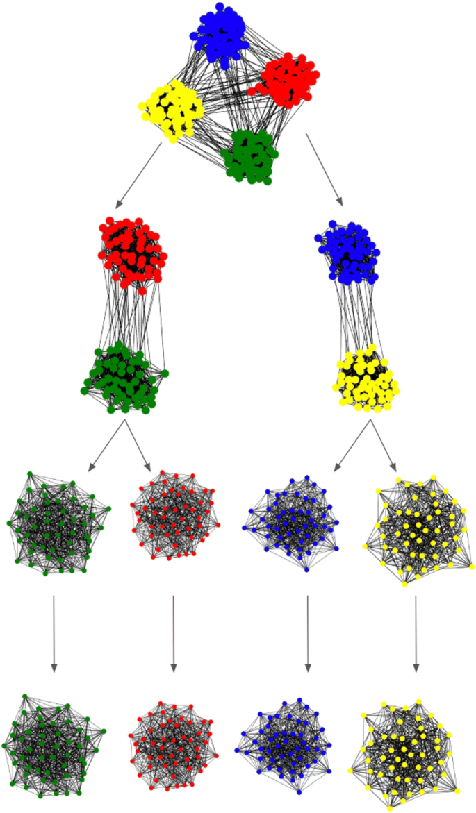
Schematic representation of the iterative procedure used by the algorithm to detect multiple communities. In this example, the top graph is a sample network with 4 communities. In the first iteration, the algorithm splits the network perfectly into two equal communities. In the next iteration, each network is split perfectly again. The algorithm terminates because the next iterations do not lead to the discovery of other sub-communities
-
2
Apply the bipartition algorithm to the graph g.
-
a
If the algorithm finds a split of g in two sets of nodes, namely g1 and g2, reconstruct each set as a graph using only nodes within the set, and only edges between pairs of nodes within the set. Place g1 and g2 into the list L.
-
b
If the algorithm finds only a set of nodes, so that no actual split was detected, g is considered as a community and placed in the list C.
-
a
-
3
Go back to point 2 until L is empty. The list of detected communities is given by C.

Learning the parameters of the noisy channel
So far, we tacitly assumed to know the values of the probabilities pin and pout. The assumption has been used in the bipartition algorithm of Radicchi (2018) when applied to instances of the stochastic block model with two communities. In practical situations, however, prior knowledge of the probabilities pin and pout is not available. These parameters should instead be learned in a self-consistent way by the algorithm relying only on information from the observed network. Here, we simultaneously propose and validate a simple learning strategy. To this end, we generate instances of the so-called Girvan-Newman (GN) benchmark graph (Girvan and Newman 2002), a variant of the stochastic model with N=128 and Q=4 communities. Different from the original version of the GN model we allow nodes to have average degree 〈k〉≠16. The average connectivity of the model is set by fixing the sum of the true parameter values \(\hat {p}_{in}\) and \(\hat {p}_{out}\), while the strength of the community structure is instead determined by their difference. We consider four different combinations \(\left (\hat {p}_{in}, \hat {p}_{out}\right)\) for the true values of the model parameters to generate four instances of the model. To each of the four instances, we apply the original algorithm with the regular starting conditions to the network using the parameters values \(\tilde {p}_{in}\) and \(\tilde {p}_{out}\). We measure the performance of the algorithm to recover the pre-imposed community structure of the graph, using normalized mutual information (NMI)
NMI is defined as the mutual information I between the predicted and true clusters normalized by the square root of the product of the individual entropies H (Strehl and Ghosh 2002; Danon et al. 2005).
In Fig. 3, we display the outcome of our tests when the community detection algorithm is applied relying on prior information given by \(\tilde {p}_{in}\) and \(\tilde {p}_{out}\). We consider only combinations \(\left (\tilde {p}_{in}, \tilde {p}_{out}\right)\) that lay in the regime of detectability (Decelle et al. 2011b). The figure shows that our algorithm reproduces accurately the community structure of the graph for several combinations \(\left (\tilde {p}_{in}, \tilde {p}_{out}\right)\). This fact happens as long as \(\left (\tilde {p}_{in}, \tilde {p}_{out}\right)\) is not too far from the ground truth \(\left (\hat {p}_{in}, \hat {p}_{out}\right)\). The finding tells us that knowing the exact value is not a necessary requirement for the correct detection of the modules; we need only a good guess of the values of the parameters. In particular, the analysis suggests a simple criterion for the choice of the parameter values pin and pout that can be used in the algorithm. We can use any combination that satisfy the equations

Learning the parameters of the noisy channel. Each subgraph report results obtained on an artificial network constructed according to a synthetic model similar to the Girvan-Newman benchmark, where N=128 are divided into Q=4 communities of equal size. Nodes within the same group are connected with probability \(\hat {p}_{in}\), while pairs of nodes belonging to different groups are connected with probability \(\hat {p}_{out}\). We consider four different combinations \(\left (\hat {p}_{in}, \hat {p}_{out}\right)\) to generate four different instances of the model. The four different instances of the model are represented in panels a, b, c, and d. Ground-truth values of \(\hat {p}_{in}\) and \(\hat {p}_{out}\) are denoted by the green star symbol in the various panels. We apply the method for community detection introduced in this paper to the graph using the parameters values \(\tilde {p}_{in}\) and \(\tilde {p}_{out}\), randomly sampled in the regime of detectability. The value of the normalized mutual information (NMI) between retrieved and ground-truth community structure is represented by the color of the various points. The green line in the plot identifies combinations of pin and pout compatible with the observed average degree 〈k〉 of the graph. The blue line is y=x, and denotes the region where community structure is present. The orange line is the detectability threshold \(\frac {N(Q-1)}{Q}\left (p_{in} - p_{out}\right) = \sqrt {\frac {N(Q-1)}{Q}\left (p_{in} - p_{out}\right)}\)
where 〈k〉 is the average degree observed in the network. The first equation imposes that the parameters pin and pout are compatible with the average degree of the observed network. The inequality appearing in the bottom of Eq. (11) is instead restricting our possibilities only in the regime of detectability (Decelle et al. 2011a). As any point in the segment determined by Eqs. (11) is equivalent in terms of performance, the values of the parameters pin and pout used by our algorithm are obtained with
where α>0 is a tunable parameter, whose value is chosen appropriately such that pin>pout≥0. In our numerical results, we set α=1.2. However, we verified that the performance of the algorithm doesn’t change if we choose small α values at random.
Results
Artificial graphs
First, we perform tests of the original and reduced versions of the algorithm on synthetic graphs with pre-imposed community structure. These are compared with 100 realizations from both the well-established methods Louvain (Blondel et al. 2008) and Infomap (Rosvall and Bergstrom 2008). In our numerical tests, we used the implementations of the two algorithms provided by the Python library igraph (2019). In particular, we use as best partition found by Louvain the community structure obtained looking at the lowest level of the multiresolution method (Lancichinetti and Fortunato 2009). We consider two different variants of the stochastic block model: the Girvan-Newman (GN) benchmark graph (Girvan and Newman 2002) and the Lancichinetti-Fortunato-Radicchi (LFR) benchmark graph (Lancichinetti et al. 2008). We measure the performance of the algorithms using NMI as a function of the community strength of the model, determined by the value of the mixing parameter \(\mu = \frac {k_{out}}{k_{out} + k_{in}}\), i.e., the ratio between external and total degree of the nodes. This parametrization allows for a direct comparison between our results on those reported in Lancichinetti and Fortunato (2009).
In Fig. 4a, we show the performance of the algorithms on the Girvan-Newman (GN) graph. The original algorithm is tested on 100 instances for each μ value. We compare results using both starting conditions. Similarly, Fig. 4b shows the results of the reduced algorithm on 100 instances of the GN graph. In the original implementation, at around μ=0.5, the performances of both algorithm reduce to 0. Both tend to outperform Infomap for large values of μ but perform worse than Louvain. In the reduced version of the algorithm, the performance of the regular implementation reduces to 0 when μ≥0.3. The random implementation is similar to Infomap and both start to drop around μ=0.4. As before, both perform worse than Louvain. The values of μ where we see a drop in performance are tantamount with the level of fuzziness where most of the algorithms start to systematically fail on the GN benchmark (Lancichinetti and Fortunato 2009). In most of the cases, either perfect communities or one large community was predicted. An interesting finding is that the reduced version of the algorithm is able to perform just as well as the original version with the regular conditions and just slightly worse with the random conditions for low values of μ.

Performance of the community detection algorithm on the Girvan-Newman (GN) benchmark graph. We plot measure values of the normalized mutual information (NMI) as a function of the mixing parameter μ of the model. a Results of the original version of the algorithm with both starting conditions; b Performance of the reduced version of the algorithm. Both of these are compared with Louvain and Infomap
Tests on the LFR graphs are reported in Fig. 5. Similar to Lancichinetti and Fortunato (2009), our tests were performed on networks with size either N=1000 or N=5000, generated under condition S, i.e., small communities with size in the range [10,50] nodes per community, or under condition B, i.e., large communities with size in the range [20,100]. In the generation of graph instances, community sizes are chosen at random according to power-law functions with exponent −1 defined over the aforementioned ranges. Node degrees are random variates extracted from a power-law degree distribution with exponent −2, such that the average degree of the nodes is 20 and maximum degree equals 50. We tested the performance of our algorithms over 100 instances of the model for each μ value. Given the high complexity of the original version of the algorithm, we could test in a systematic fashion only the performance of the reduced algorithm. The algorithm was started from both initial conditions. The results of Fig. 5 provide evidence that the algorithm is able to achieve good performance, although the ability to recover the right community structure of the model decreases to zero for a level of noise slightly smaller than those of other algorithms (Lancichinetti and Fortunato 2009).

Performance of the community detection algorithm on the Lancichinetti-Fortunato-Radicchi (LFR) benchmark graph. We display results only for the reduced version of the algorithm but with both initial conditions. As a term of comparison, we display results obtained by Louvain and Infomap in the same set of benchmark graphs. In the various panels, performance is measured in terms of normalized mutual information (NMI). This quantity is evaluated as a function of the mixing parameter μ of the model. We consider the following experimental settings: a Small communities with N=1000 nodes; b Big communities with N=1000 nodes; c N=5000 nodes with Small communities; d N=5000 nodes with Big communities
Real networks
Recently, community detection algorithms have been focusing on incorporating edge and node metadata into community formation (Newman and Clauset 2016). An interesting point in this context is understanding how much the community structure of a network is actually representative for exogenous classifications of nodes obtainable from metadata (Hric et al. 2014).
We run both versions of the algorithms 100 times on 5 well-known datasets with metadata. For each dataset, we applied three filters; splitting communities into connected components, removing duplicates, and removing singletons (Hric et al. 2014). The Zachary Karate Club network is a social network of 34 nodes and 78 edges of self reported friends (Zachary 1977). A disagreement between the two leaders led to the splitting of the club into two groups. The US College football network is a network of college football teams in which edges represent a scheduled game in the Fall of 2000 (Girvan and Newman 2002). The communities are the 12 conferences each of the teams belong to. The US Political Book network represents all books co-purchased on Amazon.com around the 2004 election in which edges are Amazon recommendations indicating co-purchases from other users while the groups represent the political leanings of the book (Liberal, Neutral, or Conservative) found by human ratings (Krebs 2008). The US Political Blog dataset is a network of hyperlinks between blogs with the groups being Conservative or Liberal (Adamic and Glance 2005). Finally, the Facebook social networks are undirected friendship networks from 97 different colleges across the US (Traud et al. 2012). We specifically use network 82 with dorms, gender, high school, and major as the communities. Due to the size, we only ran 5 iterations on the Facebook network.
Table 2 shows the performance of algorithms, under both initial conditions, on the various datasets. Performance is still measured in terms of NMI between the community structure recovered by the algorithms and the one given by the metadata. Best matches between topological communities and metadata were observed for the US College Football network, similar to Hric et al. 2014. The result is expected as college football teams play more against teams within their conference rather than teams outside their conference. Interestingly, the communities found by our algorithm seem to provide significantly higher NMI values than those obtained via Louvain and Infomap on the US Political Book and US Political Blog networks.
Conclusion
In this paper, we exploited the interpretation of the problem of defining and identifying communities in networks as a classical communication task over a noisy channel, and made use of a widely-used decoding technique to generate a novel algorithm for community detection. Although the primitive version of the algorithm was introduced in Radicchi (2018), we extended the idea in three respects. First, we generalized the algorithm, originally designed for the detection of two communities only, to the detection of an arbitrary number of communities. The generalization consists of iterating the binary version of the algorithm till convergence. Second, we accounted for the sparsity of graphs which community detection methods are usually applied to, and reduced the complexity of the algorithm from quadratic to linear. The simplification allowed us to generate a method able to deal with potentially large networks without renouncing too much to the basic principles of the original version of the algorithm. Third, we systematically tested the performance of the new algorithm on both synthetic networks and real-world graphs. These tests provided results that are consistent with what already observed in the literature for other well-established algorithms for community detection. In particular, the algorithm outperformed top community detection algorithms in tests based on the standard SBM, i.e., involving the detection of equally sized communities in graphs with homogenous degree distributions. On the basis of the performance results obtained here, we believe that our algorithm may represent an effective and efficient alternative to other methods that rely on the SBM ansatz to infer network community structure.
References
Abbe, E (2018) Community detection and stochastic block models: recent developments. J Mach Learn Res 18(177):1–86.
Abbe, E, Bandeira AS, Hall G (2016) Exact recovery in the stochastic block model. IEEE Trans Inf Theory 62(1):471–487.
Abbe, E, Sandon C (2015) Community detection in general stochastic block models: Fundamental limits and efficient algorithms for recovery In: Foundations of Computer Science (FOCS), 2015 IEEE 56th Annual Symposium On, 670–688.. IEEE.
Adamic, LA, Glance N (2005) The political blogosphere and the 2004 us election: divided they blog In: Proceedings of the 3rd International Workshop on Link Discovery, 36–43.. ACM.
Blondel, VD, Guillaume J-L, Lambiotte R, Lefebvre E (2008) Fast unfolding of communities in large networks. J Stat Mech Theory Experiment 2008(10):10008.
Clauset, A, Newman ME, Moore C (2004) Finding community structure in very large networks. Phys Rev E 70(6):066111.
Danon, L, Diaz-Guilera A, Duch J, Arenas A (2005) Comparing community structure identification. J Stat Mech Theory Experiment 2005(09):09008.
Decelle, A, Krzakala F, Moore C, Zdeborová L (2011a) Asymptotic analysis of the stochastic block model for modular networks and its algorithmic applications. Phys Rev E 84(6):066106.
Decelle, A, Krzakala F, Moore C, Zdeborová L (2011b) Inference and phase transitions in the detection of modules in sparse networks. Phys Rev Lett 107(6):065701.
Duch, J, Arenas A (2005) Community detection in complex networks using extremal optimization. Phys Rev E 72(2):027104.
Fiduccia, CM, Mattheyses RM (1982) A linear-time heuristic for improving network partitions In: Proceedings of the 19th Design Automation Conference, 175–181.. IEEE Press.
Fortunato, S (2010) Community detection in graphs. Phys Rep 486(3-5):75–174.
Friedman, J, Hastie T, Tibshirani R (2001) The Elements of Statistical Learning vol. 1. Springer.
Gallager, R (1962) Low-density parity-check codes. IRE Trans Inf Theory 8(1):21–28.
Girvan, M, Newman ME (2002) Community structure in social and biological networks. Proc Natl Acad Sci 99(12):7821–7826.
Guimera, R, Sales-Pardo M, Amaral LAN (2007) Module identification in bipartite and directed networks. Phys Rev E 76(3):036102.
Hastings, MB (2006) Community detection as an inference problem. Phys Rev E 74(3):035102.
Hric, D, Darst RK, Fortunato S (2014) Community detection in networks: Structural communities versus ground truth. Phys Rev E 90(6):062805.
Karrer, B, Newman ME (2011) Stochastic blockmodels and community structure in networks. Phys Rev E 83(1):016107.
Kernighan, BW, Lin S (1970) An efficient heuristic procedure for partitioning graphs. Bell Syst Tech J 49(2):291–307.
Krebs, V (2008) A network of books about recent us politics sold by the online bookseller amazon.com. Unpublished http://www.orgnet.com. Accessed 1 Oct 2018.
Krzakala, F, Moore C, Mossel E, Neeman J, Sly A, Zdeborová L, Zhang P (2013) Spectral redemption in clustering sparse networks. Proc Natl Acad Sci 110(52):20935–20940.
Lancichinetti, A, Fortunato S (2009) Community detection algorithms: a comparative analysis. Phys Rev E 80(5):056117.
Lancichinetti, A, Fortunato S, Radicchi F (2008) Benchmark graphs for testing community detection algorithms. Phys Rev E 78(4):046110.
MacKay, DJ, Mac Kay DJ (2003) Information Theory, Inference and Learning Algorithms. Cambridge university press.
MacKay, DJ, Neal RM (1996) Near shannon limit performance of low density parity check codes. Electron Lett 32(18):1645.
Mossel, E, Neeman J, Sly A (2018) A proof of the block model threshold conjecture. Combinatorica 38(3):665–708.
Nadakuditi, RR, Newman ME (2012) Graph spectra and the detectability of community structure in networks. Phys Rev Lett 108(18):188701.
Newman, ME (2004) Fast algorithm for detecting community structure in networks. Phys Rev E 69(6):066133.
Newman ME (2006a) Finding community structure in networks using the eigenvectors of matrices. Phys Rev E 74(3):036104.
Newman ME (2006b) Modularity and community structure in networks. Proc Natl Acad Sci 103(23):8577–8582.
Newman, ME (2013) Community detection and graph partitioning. EPL (Europhys Lett) 103(2):28003.
Newman, MEJ, Clauset A (2016) Structure and inference in annotated networks. Nat Commun 7:11863.
Newman, ME, Girvan M (2004) Finding and evaluating community structure in networks. Phys Rev E 69(2):026113.
Newman, ME, Leicht EA (2007) Mixture models and exploratory analysis in networks. Proc Natl Acad Sci 104(23):9564–9569.
Peel, L, Larremore DB, Clauset A (2017) The ground truth about metadata and community detection in networks. Sci Adv 3(5):1602548.
Peixoto, TP (2013) Parsimonious module inference in large networks. Phys Rev Lett 110(14):148701.
Peixoto, TP (2014) Hierarchical block structures and high-resolution model selection in large networks. Phys Rev X 4(1):011047.
Peixoto, TP (2018) Bayesian stochastic blockmodeling. In: Doreian P, Batagelj V, Ferligoj A (eds)Advances in Network Clustering and Blockmodeling.. Wiley, New York. arXiv preprint arXiv:1705.10225.
(2019) python-igraph. http://igraph.org/python. Accessed 10 Jan 2019.
Radicchi, F (2013) Detectability of communities in heterogeneous networks. Phys Rev E 88(1):010801.
Radicchi, F (2014) A paradox in community detection. EPL (Europhys Lett) 106(3):38001.
Radicchi, F (2018) Decoding communities in networks. Phys Rev E 97(2):022316.
Rosvall, M, Bergstrom CT (2008) Maps of random walks on complex networks reveal community structure. Proc Natl Acad Sci 105(4):1118–1123.
Shannon, CE (2001) A mathematical theory of communication. ACM SIGMOBILE Mob Comput Commun Rev 5(1):3–55.
Strehl, A, Ghosh J (2002) Cluster ensembles—a knowledge reuse framework for combining multiple partitions. J Mach Learn Res 3(Dec):583–617.
Traud, AL, Mucha PJ, Porter MA (2012) Social structure of facebook networks. Phys A Stat Mech Appl 391(16):4165–4180.
Zachary, WW (1977) An information flow model for conflict and fission in small groups. Anthropol Res 33(4):452–473.
Zhou, H (2003) Distance, dissimilarity index, and network community structure. Phys Rev E 67(6):061901.
Acknowledgments
Not Applicable.
Funding
FR acknowledges support from the National Science Foundation (CMMI-1552487) and from the US Army Research Office (W911NF-16-1-0104).
Availability of data and materials
The code and the datasets used in this analysis are available in a Github repository at https://github.com/kbathina/Error-decoding-community-detection.
Author information
Authors and Affiliations
Contributions
Both authors conceived and designed the work, and wrote the manuscript. KB performed numerical simulations. Both authors read and approved the final manuscript.
Corresponding author
Ethics declarations
Competing interests
The authors declare that they have no competing interests.
Publisher’s Note
Springer Nature remains neutral with regard to jurisdictional claims in published maps and institutional affiliations.
Rights and permissions
Open Access This article is distributed under the terms of the Creative Commons Attribution 4.0 International License (http://creativecommons.org/licenses/by/4.0/), which permits unrestricted use, distribution, and reproduction in any medium, provided you give appropriate credit to the original author(s) and the source, provide a link to the Creative Commons license, and indicate if changes were made.
About this article

Cite this article
Bathina, K.C., Radicchi, F. Error-correcting decoders for communities in networks. Appl Netw Sci 4, 9 (2019). https://doi.org/10.1007/s41109-019-0114-7
Received:
Accepted:
Published:
DOI: https://doi.org/10.1007/s41109-019-0114-7